Application notes


Technical notes
Ask an engineer


Publications
United States (EN)
Select your region or country.
A technical guide to silicon photomultipliers (MPPC) - Section 4
Ardavan Ghassemi, Hamamatsu Corporation
Kota Kobayashi & Kenichi Sato, Hamamatsu Photonics K.K.
January 11, 2018
Section 4. MPPC characterization measurements
Sometimes referred to by other terms such as a datapoint, a sampling, a reading, or an event, a measurement is a single experimental attempt [temporally (per a duration of time) and spatially (per a detector channel and within its physical size and field-of-view)] to quantify an optical signal.
The result of a measurement is thus a piece of quantitative data that represents essential information about the true signal. Measurement is a very fundamental and seemingly simple concept, so why is it explored here? There are 3 important points to keep in mind:
- Measurement frequency: Understanding the required bandwidth for a measurement is of paramount importance to proper identification and definition of an application’s requirements and in order to compare those requirements with characteristics of candidate photodetectors. Fundamentally, based on Nyquist’s sampling theorem, the sampling frequency must be at least twice the measurement frequency, which in turn would be equal to the frequency of the signal’s highest-frequency component that is intended to be detected. Furthermore, as discussed before, a readout amplifier circuit’s cutoff frequency at -3 dB should be designed to be at least twice that of the measurement frequency (but as a general rule of thumb, 4 times is an advisable design target).
For better illustration, the following examples portray cases in which a detrimental bandwidth mismatch is present:
- Using an amplifier with a cutoff frequency of 1 MHz to measure pulses with frequency of 900 kHz and rise/fall times of 1 μs.
- Using an imager with a spatial resolution of 10 lp/mm to contact-image a min. feature size of 20 μm. [Reason: 10 lp/mm is theoretically able to observe a min. feature size of 1 mm /(2 × 10) = 50 μm]
- Using an oscilloscope with a sampling rate of 150 MHz to look for multiple randomly-occurring events with durations of 10 ns each (Reason: 150 M < 2 × 1/10 n = 200 M).
- Measurement resolution and range: Besides measurement frequency, the resolution of the measurement instrumentation in its ability to accurately resolve the smallest expected quantity of or change in the parameter (that is to be measured) over the full range of its expected values is also of great importance. The following are examples in which there is a detrimental mismatch between signal characteristics and measurement resolution and range:
- Using an 8-bit digitizer with a conversion factor of 500 ke-/LSB to plot pulse height distribution for up to 150 p.e. pulses of a MPPC at gain = 106 (Reason: 150 × 106 / 5 × 105 = 300 > 28).
- Using a detector with a rise time of 10 ns to discriminate the pulse shapes of 2 signals with rise times of 1 ns and 8.5 ns.
- Using a spectrometer with a resolution of 30 nm to distinguish emission or excitation peaks 10 nm apart.
- Using a 16-bit/sample ADC with a bit rate of 50 Mbps to record the output waveform of an MPPC with a dark count rate of 4 Mcps for under dark conditions. (Reason: 50 M / 16 < 4 M)
- Normalizations: While some signal characteristics (like amplitude, timing or frequency) can be appropriately obtained from measuring a single parameter (whether once or a multitude of times), others (like flux or power) would by definition include normalizations to time and/or spatial information and hence require measurements of 2 or more parameters in order to be quantified.
These differences are important, since a typical instrument designer is naturally concerned with the performance of her overall instrumentation: she could be designing for an application condition that combines a series of measurements and contains one or more normalizations instead of consisting of a single parameter alone. In order to assess a photodetector’s suitability for a given application, one must bear that in mind and see how the way detector characteristics have been specified compares with the designer’s intended application conditions and target requirements.
Towards that, one would begin by finding out to what temporal or spatial parameters a stated application condition might have been normalized; when in doubt, one should make sure about the dimension or unit of the application condition in question. Furthermore, it is also important to understand the scope of those normalizations.
For example, one needs to examine whether the incident light “power” is applied to the entirety of a detector’s photosensitive area or normalized to pixel count or unit of area. As another example, it is important to verify whether peak power or average power is meant when a reference to incident light “power” is made; peak and average power have different temporal normalizations in that the former is the ratio of energy content of a single pulse to the time duration of that pulse while the latter takes the time in between consecutive pulses into account. As a further example, if various spectral band components of a broad spectrum of light are to be detected by different detector channels separately (applicable to 1D or 2D serial- or parallel-readout multichannel detectors), performance of each detector channel must be assessed independently in accordance to its particular expected input light signal conditions.
With the above caveats in mind, we proceed to introducing methods of measuring MPPC characteristics. In what follows, we will focus on the characterization of Hamamatsu’s S13360-3050CS as an example, but please be assured that these measurement methods can be adapted to other MPPC models with little or no adjustments.
Before we begin, however, let’s briefly discuss the choice of a suitable power supply to bias the MPPC. At Hamamatsu Photonics, we typically utilize a source meter to bias the MPPC, since it allows us to control the applied voltage via a PC connection and also to set a max. voltage of 80 V for safe biasing of the MPPC. Furthermore, a source meter enables automated I-V curve characterization and can thus be used in QC screening of mass-produced parts. Therefore, despite its relatively high cost, a source meter is recommendable as a suitable biasing solution in performing the measurements described hereinafter.
4-1. Gain and breakdown voltage (VBR) measurement
- Measurement principle: MPPC gain is the factor by which Geiger-mode avalanche (whether initiated by the photoelectric effect or thermal carrier excitation) multiplies the initiating electron to form the MPPC’s output charge per avalanche. Following the mechanism that we explained in Section 1, that gain is proportional to overvoltage (Vover), which is the difference between the bias voltage applied to the MPPC and the MPPC’s inherent breakdown voltage (VBR).
The simplest measurement of VBR can be derived from the x-intercept of a MPPC’s gain vs. bias voltage plot. Assuming a proportionality factor of A between gain and overvoltage, we can say Gain = A x Vover = A x (Vbias - VBR), and at the gain-voltage plot’s x-intercept (at which Gain = 0), Vbias thus corresponds to the breakdown voltage.
Determining the VBR of MPPC before beginning other measurements is practically beneficial and recommendable. Most MPPC characteristics whose measurement we are going to introduce in this section, namely photon detection efficiency, dark count rate, prompt or delayed crosstalk probability, and afterpulse probability, are dependent on Vover. Additionally, VBR differs between each and every pair of MPPCs even if they are the same product – for example, amongst a small batch of S13360-3050CS, VBR of each is different from the rest; operating them at the same applied bias voltage would likely result in differing characteristics. It is thus recommended to compare or calibrate the characteristics of MPPCs at the same overvoltage (or the same gain if practical).
- Measurement setup: Figure 4-1 shows the gain measurement setup. In this setup, the MPPC is placed inside a dark box and electrically connected to it (if metallic) via a common ground in order to decrease the parasitic impedance that forms between them. Output of the charge amplifier goes to a shaping amplifier, which is followed by a MCA. Finally, a dedicated FPGA circuit sends the MCA output to a PC through a USB connection. We analyze the data coming from the MCA with a LabVIEW software program in this setup.
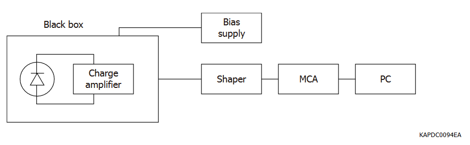
Figure 4-1 Gain measurement setup
- Measurement procedure: In our setup, the MCA output is used to produce a histogram of the shaping amplifier’s output pulses; this histogram would consist of pulse count and digitized pulse height (proportional to the MPPC’s output charge) as its y and x axes, respectively. Figure 4-2 shows an example of this histogram. As shown, the histogram has several peaks, which correspond to (from left to right) the noise pedestal (population of readout noise pulses) and populations of 1 p.e., 2 p.e., ... pulses of the MPPC. Based on the properties of these peaks, we can compute the net output charge corresponding to a 1 p.e. pulse by calculating the peak-to-peak interval between any two consecutive peaks (excluding the pedestal) along the x-axis after which we convert the interval value (in digital counts [LSB]) to equivalent charge amount based on the charge amplifier’s gain [V/C] and the MCA’s A/D conversion factor [LSB/V]. This 1 p.e. equivalent charge is, by definition, equal to the gain of the evaluated MPPC at the applied bias voltage. We repeat this measurement process for various applied voltages to obtain the gain-voltage plot. We then perform linear fitting on the resulting plot; the x-intercept of the fitted line represents VBR of the MPPC under evaluation.
It is noteworthy to point out a potential pitfall in performing this measurement: the MPPC output pulse populations must be sufficiently large to be statistically significant in order to create a meaningful histogram. This condition could be difficult to attain for low overvoltage levels or if the MPPC’s dark count rate is too small. In such scenarios, low-intensity illumination of MPPC photosensitive area should be utilized to increase the output pulse counts.
- Measurement result: Figure 4-3 shows the gain-voltage plot and its linear fit for S13360-3050CS. From this plot, we conclude that VBR of this MPPC is 51.29 V.
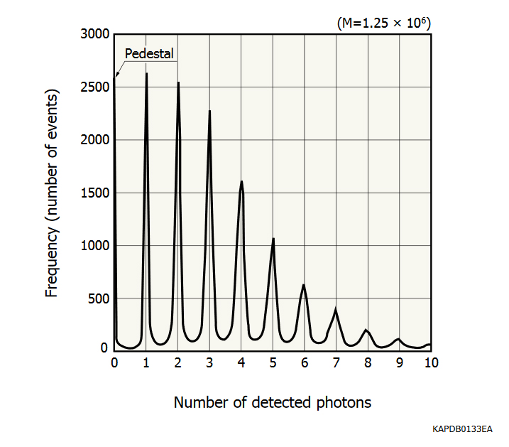
Figure 4-2 Histogram example of shaping amplifier’s output pulse
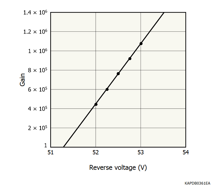
Figure 4-3 Gain vs. voltage plot example (S13360-3050CS)
4-2. Breakdown voltage measurement by obtaining Vpeak from I-V curve
- Measurement principle: There is another way of obtaining MPPC’s VBR that is useful when evaluating many MPPC units of the same type. We use this measurement method in the mass inspection of our MPPC products.
Vpeak is defined as the inflection point of log(I) vs. V curve. The critical property of Vpeak is that the subtraction Vpeak - VBR depends only on the type of MPPC and not on the actual value of VBR. Combined with the fact that measuring the I-V curve only around Vpeak is less cumbersome than measuring the gain-voltage plot, this measurement method is highly efficient for evaluating VBR for a large batch of MPPCs.
To illustrate with an example, let us assume that we want to evaluate VBR values of 100 units of S13360-3050CS. Measuring the gain-voltage plot 100 times for all units would be very demanding, so we instead obtain VBR of just one unit, considering that measuring gain-voltage plot only one time is not too much of a burden. For the same unit, we then obtain its Vpeak by the method to be described here shortly, so that we can calculate the value of (Vpeak − VBR) from these two measurement results. This value is common amongst all 100 units of S13360-3050CS in our hypothetical batch, and we can calculate VBR of the remaining 99 units by measuring their individual I-V curves and obtaining their particular Vpeak values.
- Measurement setup: Figure 4-4 shows the Vpeak measurement setup. The setup is the same as that of gain measurement but with the key differences being utilization of a stable light source (such as an LED) and a different output readout scheme. In this setup, we directly connect the MPPC to a source meter and simply read out the MPPC’s output current. We repeat this readout for various applied voltages to obtain the I-V curve.
We transfer this I-V curve data from the source meter to a PC in order to perform I-V curve analysis and obtain the Vpeak of each MPPC under evaluation.
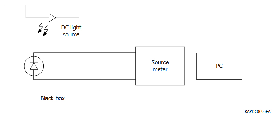
Figure 4-4 Vpeak measurement setup
- Measurement procedure: Figure 4-5 shows a measured I-V curve of S13360-3050CS under various luminance levels coming from the light source. Under dark condition, the I-V curve comprises bulk current and surface leakage current. The latter strongly affects the I-V curve’s baseline under dark condition and the resulting Vpeak. By illuminating MPPC with the light source, however, we can ignore the baseline and calculate the Vpeak reliably. In practice, one should experimentally determine the suitable LED luminance by repeating the I-V curve measurement for various light levels while avoiding excessive illumination of the MPPC.
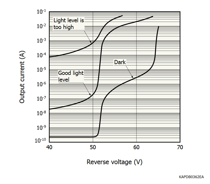
Figure 4-5 I-V curve example of Vpeak measurement
- Measurement result: Table 4-1 shows the Vpeak measurement results for three units of S13360-3050CS. For reference, measured VBR of each of those MPPCs (via the x-axis intercept method) has also been listed. As you can see, the difference Vpeak − VBR has the same value amongst all three.
Table 4-1 Vpeak (and VBR) measurement result for 3 pcs of S13360-3050CS
| Sample no. | 1 | 2 | 3 | Unit |
|---|---|---|---|---|
| Vpeak | 51.47 | 51.57 | 51.87 | V |
| VBR | 51.29 | 51.41 | 51.70 | V |
| Difference | 0.18 | 0.16 | 0.17 | V |
4-3. Photon detection efficiency (PDE) vs. bias voltage measurement
- Measurement principle: A key aspect of measuring MPPC’s PDE is the exclusion of correlated noise (optical crosstalk and afterpulses) from the measured data. While several such techniques have been devised over the recent years, the best-known MPPC PDE measurement technique (also utilized by Hamamatsu) has been described extensively in [11]. We will provide an overview of that technique as performed by Hamamatsu in this subsection.
In simple terms, the aforementioned technique relies on measuring the amplitudes of MPPC output pulses (instead of output current), plotting a pulse height histogram, and then calculating the ratio of non-photon (< 1 p.e. in height) event count (also known as the pedestal event count and noted as Nped in [11]) to total event count (= Nped + N≥1p.e. and noted as Ntot in [11]). This ratio is not affected by crosstalk and afterpulses because correlated noise does not occur in absence of signal detection; it only appears in correlation with genuine (thermal or photoelectric) events of 1 p.e., 2 p.e., ... in height.
- Measurement setup: Figure 4-6 shows the PDE measurement setup.
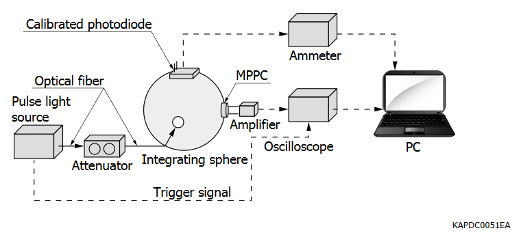
Figure 4-6 Hamamatsu’s PDE measurement setup
The following are typical examples of instruments that can be used in this measurement setup:
Pulse light source: PLP-10 (Hamamatsu)
Wavelength: 408 nm (several other wavelengths such as 655 nm, 851 nm, etc. are also available)
Pulse width: 88 ps FWHM (wavelength dependent)
Optical attenuator6: DA-100-3U-850-50/125-M-35 (OZ Optics)
Integrating sphere: 3P-GPS-033-SL (Labsphere)
Power meter: 2936-R (Newport)
Bias supply: GS610 (Yokogawa) or 2636B (Keithley) and the like
Amplifier: Linear amplifier (internal product and not for sale), bandwidth: 450 MHz
Oscilloscope: SDA 760Zi (LeCroy)
Measurement software program is written in LabVIEW 2010.
6 The listed optical attenuator is designed for an attenuation wavelength of 850 nm. When the optical signal wavelength is different from the attenuator’s design wavelength, the actual attenuation level would differ from what the user sets the attenuator to operate at. Nevertheless, for the purpose of this measurement, we do not need to know the attenuation level since we can measure the attenuator’s output (as the number of photons that are illuminated onto the MPPC) by the power meter. In that sense, we only use the attenuator to adjust the amount of light incident onto the MPPC; how much light is lost (between the source and the attenuator’s output) is irrelevant to this measurement.
The pulsed light source used in this measurement should emit monochromatic light and must have a pulse width shorter than the MPPC rise time (which is on the order of a few nanoseconds).
In utilizing the integrating sphere, we mount the MPPC and the power meter’s photodiode head on two output ports of the sphere. To hold it on the output port, the MPPC is mounted using a fixture with a small aperture radius (0.5 mm or 0.3 mm depending on the MPPC’s photosensitive area in order to ensure the illumination of the MPPC photosensitive area only).
The ratio of output light levels of the sphere’s two ports should be measured in advance by mounting the same photodiode head on each port and dividing the resulting power meter outputs. It should be emphasized that light intensity in determining the output power ratio of the sphere’s ports should be high enough to allow for the power meter’s photodiode head to detect it with good accuracy through the small aperture of MPPC’s fixture. When using a pulsed light source as in our case, higher light intensities can be achieved by increasing the light pulse frequency.
To ensure high S/N for good measurement accuracy, the output amplifier used to read the MPPC must have relatively low levels of noise. Since an amplifier’s noise performance and its bandwidth are competing factors, it is acceptable to compromise on the bandwidth even if that would result in the distortion of the MPPC output pulse shape.
For digitization and analysis of the linear amplifier’s output pulses, we use the oscilloscope SDA 760Zi (LeCroy), which has the capability to perform PHA/PHD (i.e. create pulse height analysis/distribution histograms) at a high data throughput.
- Measurement procedure: Figure 4-7 shows a flowchart of our PDE measurement program’s underlying algorithm. We wrote this program to automatically measure MPPC’s PDE vs. bias voltage.
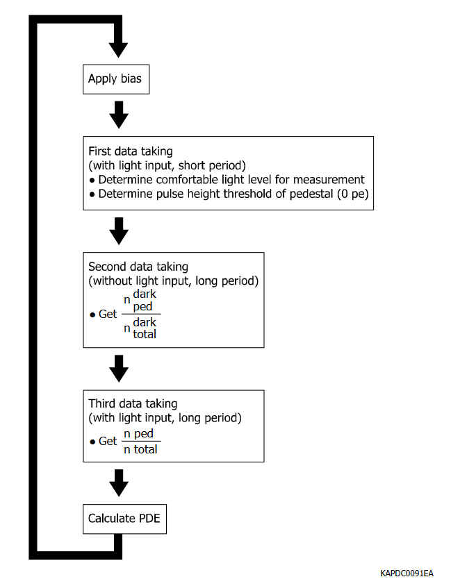
Figure 4-7 Flowchart of our PDE measurement program’s algorithm
The flowchart loop begins with setting an initial bias voltage, which must be controlled by a temperature-compensation scheme if a temperature-controlled enclosure or ambient environment is unavailable. Then, we proceed to the main measurement procedure that comprises three data taking steps: the first measures the light intensity incident onto the MPPC and determines the Nped threshold while the following two steps measure Nped.
For determining Nped in the following two steps, we use simpler criteria (than what has been described in [11]) by counting the number of events below the threshold set by Step A. This approach is suitable when there is good separation between discrete p.e. peaks and a reasonably high (≥ 2) peak-to-valley (P/V) ratio exists between 0 p.e. and 1 p.e. peaks and the valley between them. If such distinct separation between peaks is not attained, the 0 p.e. peak can be fitted to a Gaussian distribution curve with the area under it calculated as described in [11]. For the case of S13360-3050CS, as Figure 4-8 shows, our simple method can be reliably used. This measurement is not intended to take Nped / Ntot precisely, and a short measurement time period is acceptable. In this case, we set it to 10 seconds. If the light level is too low or too high to measure the 0 p.e. ratio effectively for the following measurement, we change the light intensity by changing the optical attenuation level and repeat collecting the data until the light intensity becomes suitable for the following steps.
Step B is for measuring Npeddark / Ntotdark in dark condition. Now, we set the light attenuation level to the maximum (40 dB in this example) to ensure that the MPPC is practically under dark condition. The time period of data taking should be long enough to exclude the statistical fluctuation of 0 p.e. events, and we thus set the time to 2 minutes in this step.
Step C is for measuring Nped / Ntot. We set the light attenuation to the level utilized in Step A but then take the data with a comparatively long period (2 minutes – same as Step B). At the same time, we obtain the number of input photons (incident onto the MPPC) per light pulse (nin) from the average value of power meter output during data collection as divided by the light pulse rate.
After these data collection steps, we finally calculate the PDE value for this bias voltage using Npeddark / Ntotdark, Nped / Ntot and nin. Subsequently, we return to the beginning of the flowchart loop and repeat this procedure for the next bias voltage.
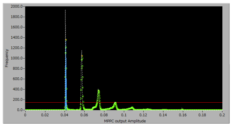
Figure 4-8 MPPC characterization and measurement program
- Measurement result: Figure 4-9 shows the result of measuring S13360-3050CS’s PDE with our setup.
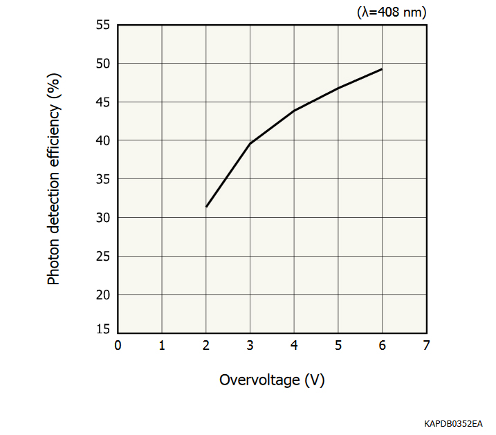
Figure 4-9 A PDE measurement example (S13360-3050CS)
4-4. Dark count rate (DCR) and prompt crosstalk measurement using counter and CR filter
- Measurement principle: In this measurement, our goal is to collect the data for the step plot of DCR vs. discriminator threshold that is shown in Figure 1-26 of Section 1-3. From that plot, DCR can be obtained as the value of the first plateau, and the prompt crosstalk probability can be calculated by the ratio [(second plateau) / (first plateau)].
It is important to note, however, that pulse pileup, which is the overlapping of output pulses described in Section 2, can have a degrading effect on the accuracy of this measurement.
Figure 4-10 shows the effect of pulse pileup. In ideal cases, MPPC output pulses are completely separated, and from the view of a counter, these pulses have completely discrete levels of pulse height with little randomness derived from gain fluctuation and white noise. However, if an MPPC has high DCR and/or long fall time because of large terminal capacitance and/or high probability of delayed crosstalk and afterpulses, pulse pileup under dark conditions can take place as shown in the lower part of Figure 4-10.
Due to pulse pileup, a lower than actual number of MPPC output pulses would be counted, and the resulting steps of DCR vs. discriminator threshold plot become less steep, hindering the accurate determination of the number of counts of each plateau. Furthermore, groupings of pulses can be counted as “one big pulse”, especially in the case of < 1 p.e. pulses whose population would be greater, and thus, the count of pulses at low threshold becomes smaller than the actual value. Generally speaking, these effects make prompt crosstalk probability larger than the actual value because the count of pulses exceeding the 0.5 p.e. threshold in height is diminished while the count of pulses whose heights exceed the 1.5 p.e. threshold is inflated.
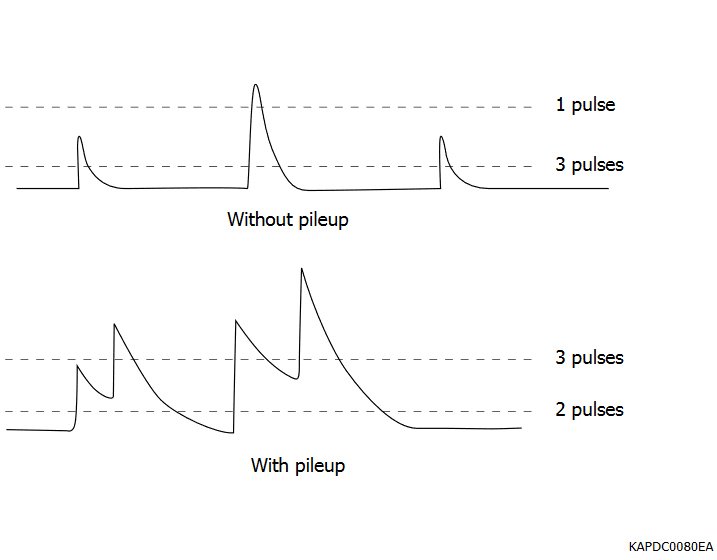
Figure 4-10 Pulse pileup effect on measurements using counter
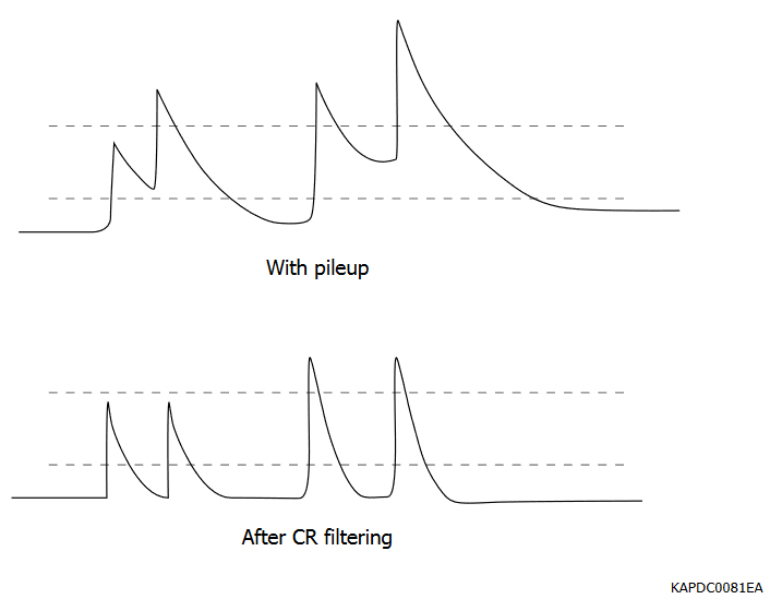
Figure 4-11 Pulse pileup reduction using CR filter
To exclude this degradation of measurement by pulse pileup, we can use a high-pass filter for pulse shaping after the linear amplifier’s output. As a result, output pulse widths become narrower and pileup is decreased as shown in Figure 4-11.
- Measurement setup: Figure 4-12 shows the measurement setup.
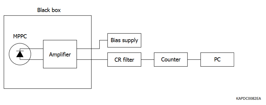
Figure 4-12 DCR measurement setup using counter and band-pass filter
Amplifier: Linear amplifier (internal product and not for sale), bandwidth: 1 GHz
High-pass filter: internally made and caged in test box
Counter: 53131A (Agilent)
In this setup, the linear amplifier should have sufficient bandwidth to replicate the MPPC rise time (as the highest-frequency component of the MPPC output) in order to effectively reject the pulse pileup effect. For a detailed explanation on how to determine the readout amplifier’s optimal bandwidth, please refer to Section 2.
The time constant of high-pass filter should be set according to the pulse shape of the MPPC that you want to evaluate. For the purpose of characterizing S13360-3050CS, we use the high-pass filter with 100 pF capacitor and 51 Ω resistor.
As explained in Section 1, the high-pass filter decreases the output pulse height and so extra amplifier gain might be required for effective pulse output measurement. In that case, one solution is implementing another linear amplifier between the first stage and the high-pass filter. We use Mini-Circuit ZX60-14012L-S+ for this purpose.
- Measurement procedure: Figure 4-13 shows the flowchart of this measurement program’s algorithm.
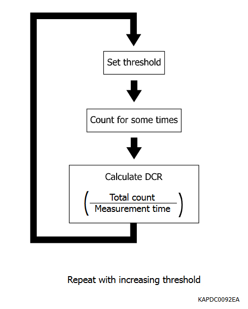
Figure 4-13 Flowchart of DCR and prompt crosstalk measurement program using a counter
The counting integration time for each threshold value should be reasonably large enough to exclude statistical fluctuation of the measured count. For the case of S13360-3050CS, we set the integration time to 2 seconds. If DCR of the measured MPPC is small because of its small photosensitive area or low temperature or other factors, integration time should be set longer.
- Measurement result: Figure 4-14 shows the measurement result for S13360-3050CS with and without high-pass filter. The high-pass filter’s effect is clearly appreciable. Figure 4-15 shows the step plot for various overvoltages (with high-pass filter); we can see the increases in gain, DCR and prompt crosstalk probability. Figure 4-16 shows the DCR and prompt crosstalk probability obtained by this measurement.
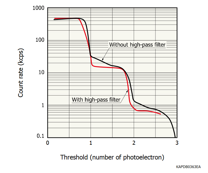
Figure 4-14 Comparison of the data with and without high-pass filter (S13360-3050CS)

Figure 4-15 Measurement results using counter (S13360-3050CS)
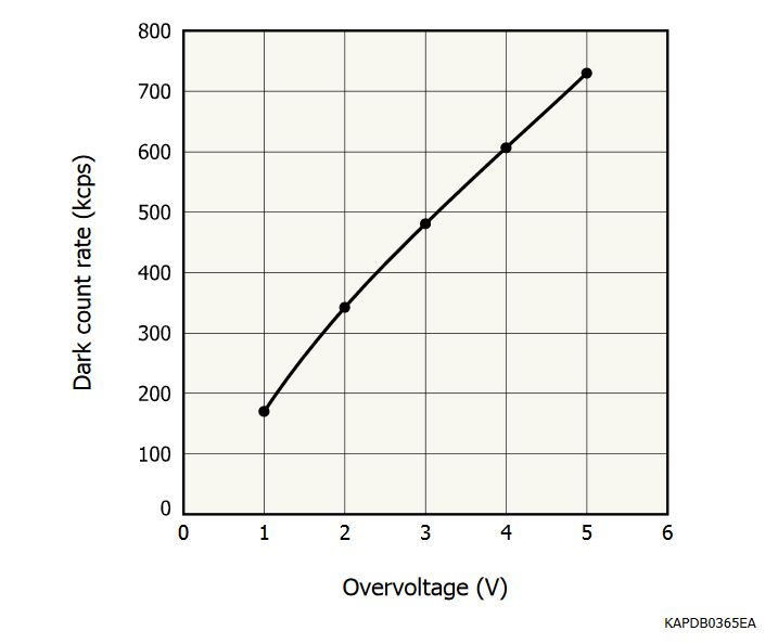
Figure 4-16a DCR and prompt crosstalk measurement results (S13360-3050CS)
(a) Dark count rate vs. overvoltage
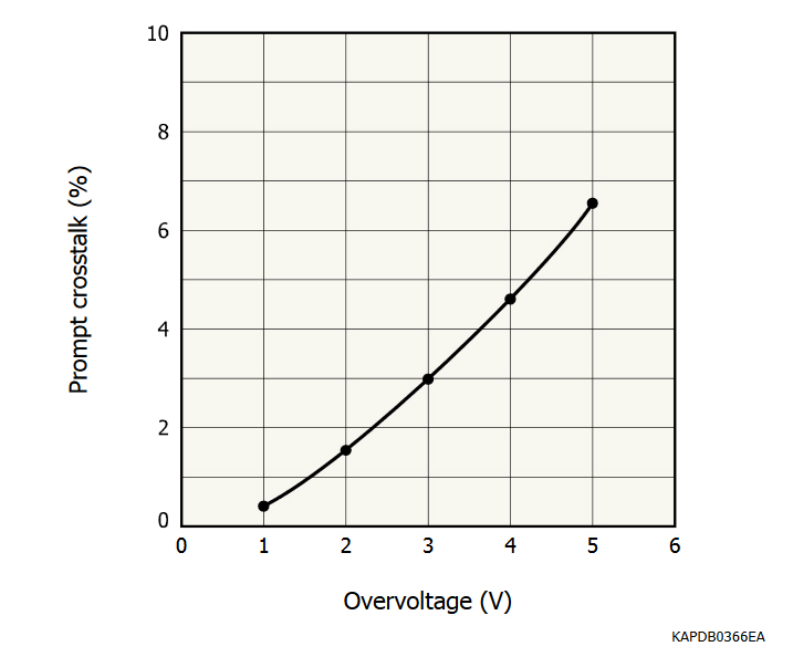
Figure 4-16b DCR and prompt crosstalk measurement results (S13360-3050CS)
(b) Prompt crosstalk vs. overvoltage
4-5. Measurement of various MPPC characteristics using digitizer and digital pulse processing
- Measurement principle: In this measurement, we measure various MPPC characteristics by detecting MPPC output events with digitizer and software processing of the resulting data. This approach is commonly referred to as digital pulse processing (DPP).
For the sake of our discussion, we denote an “event” as data obtained within a time window that would contain MPPC output pulses (one or more) of any height. Specifically speaking, in the case of S13360-3050CS, the full width of a single output pulse is about 200 ns; we digitize the output waveform during a time window on the order of microseconds for DCR measurement and on the order of hundreds of nanoseconds for other measurements. You should choose the time window according to your measurement objective. A smaller time window leads to the reduction of valid events and consequently to the diminishment of afterpulse output whereas a larger time window results in a larger data size for one event and thus a decrease in measurement throughput.
In a manner similar to the hardware solution (high-pass CR filter) described earlier, we resolve the issue of pulse pileup through software processing of an MPPC event using a deconvolution filter. The basic concept of this method is well-known in the digital image processing field and described in references such as [12] while its practical application to the photosensor signal processing is described in [13] (in Japanese). There are other solutions for pulse pileup rejection such as simply differentiating the output and suppressing baseline discrepancy as described in [14].
A conceptual illustration of the deconvolution filter is shown in Figure 4-17. We assume that the MPPC output can be represented by the convolution of Dirac delta-function output events and the 1 p.e. MPPC waveform. The delta-function event is free from pileup since each such pulse would have a very sharp and distinct shape. If we define the specific shape of the delta waveform and measure the 1 p.e. waveform of the MPPC under measurement, we can mathematically compute the deconvolution filter that converts the real MPPC output events to delta-function events and thus reject the pulse pileup effect. Detailed mathematical explanation of how the deconvolution filter is computed has been provided in [13] and [14].
In addition to the deconvolution filter, we use another filter to reduce white noise, which disturbs the detection of delta-function peaks. Hamamatsu’s choice of such filters is the Wiener filter that determines the reduction in pulse height of a 1 p.e. MPPC output pulse as a function of frequency by computing the Fourier transform of the 1 p.e. waveform in frequency domain after white noise filtration. Other methods are also effective; one of the simplest is to apply a low-pass filter to the event or equivalently set the oscilloscope bandwidth to a small value compared to the highest-frequency component of a 1 p.e. MPPC so that white noise can be filtered out while the MPPC output pulse maintains its amplitude.
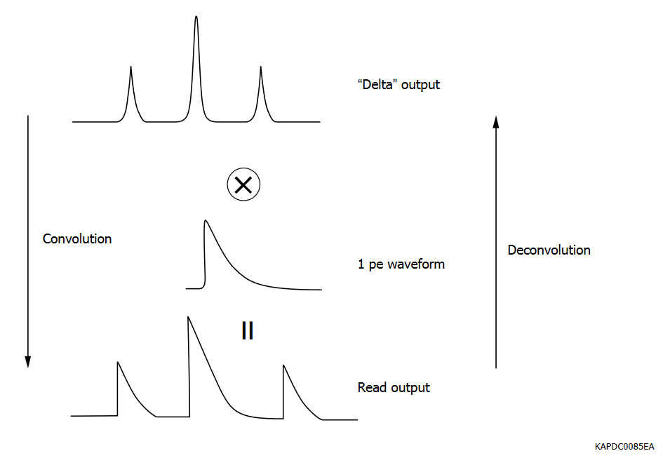
Figure 4-17 Basic concept of waveform deconvolution
- Measurement setup: Figure 4-18 shows the measurement setup for this method. The MPPC is placed in a black box, and we proceed to recording the dark output events.
We use the oscilloscope as a digitizer in this measurement; board-level digitizers such as Flash ADCs are also suitable if they have sufficient node sensitivity, bandwidth, and sampling rate for precisely recording MPPC output pulse shapes. For our purpose, the 1 GHz bandwidth and 10 GS/s sampling rate of oscilloscope DPO7104 (Tektronix) is adequate.
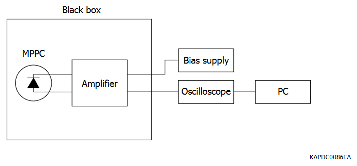
Figure 4-18 Measurement setup using a digitizer (oscilloscope)
- Measurement procedure: Before starting the data collection, we first form the deconvolution and Wiener filters and then combine them.
Figure 4-19 shows how to make the deconvolution filter.
First, we obtain the MPPC’s 1 p.e. waveform (the method of obtaining it is explained in the next subsection), and we then define the delta-function pulse shape based on the obtained 1 p.e. waveform. We afterwards use the Blackman window function7 as the delta function’s shape and determine the window’s optimal width by setting various widths and checking the deconvolution result for each of them. We then perform the Fourier transform operation on each waveform and calculate the ratio of its intensity for every frequency and obtain the deconvolution component of the filter.
7
We then proceed to building the Wiener component of the filter by using the Fourier form of 1 p.e. pulse. We first obtain the white noise by recording the output waveform while applying a bias voltage slightly below the MPPC’s breakdown voltage and calculating the Fourier transform of the resulting noise waveform. Using the two Fourier functions, we then calculate their power ratio as described in Figure 4-19 to obtain the Wiener component of the filter.
Finally, we form the product of deconvolution component and Wiener component and perform inverse Fourier transform on the product. The resulting waveform is the pulse processing filter we want.
In this example, we use LabVIEW’s library functions for the Fourier and inverse Fourier transform operations. You can use other math library functions prepared by other programming languages (such as MATLAB); there should be no differences in the results.
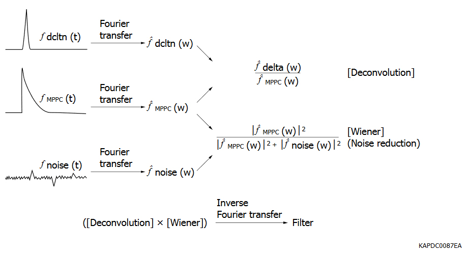
Figure 4-19 Mathematical basis for creating a filter to cancel the effects of MPPC output pulse pileup and white noise
After creating the filter, we take a MPPC output event and convolute the entire event with the filter to obtain the delta pulse output. The effect of deconvolution is shown in Figure 4-20, and an example of it for S13360-3050CS is shown in Figure 4-21.
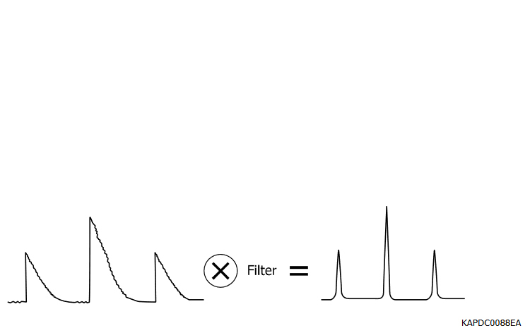
Figure 4-20 “Delta” output with white noise reduced in a single step using the filter we made
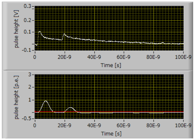
Figure 4-21 Deconvolution example (S13360-3050CS)
Processing the filtration’s output can be performed by two approaches, which we now proceed to explain.
DCR and prompt crosstalk measurement: In the first approach, the digitizer is triggered arbitrarily; an example of the trigger source would be 417 NIM pocket pulser (made by Phillips Scientific).
Figure 4-22 shows the concept of how to obtain DCR and prompt afterpulse probability in this measurement. To each MPPC output event recorded, we apply the aforementioned filtration in order to obtain a delta-function output event and then count the number of pulses in the event with a 0.5 p.e. discriminator threshold. The DCR can thus be obtained as the following simple ratio:
[(Number of pulses)/(Event time window)].
The prompt crosstalk can also be obtained easily by counting the number of pulses with a 1.5 p.e. threshold during the same time window and calculating the following ratio: [(number of >1.5 p.e. pulses)/(number of >0.5 p.e. pulses)].

Figure 4-22 The principle of DCR measurement method using a digitizer
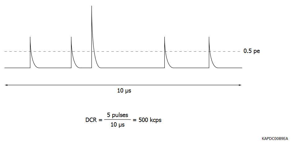
Figure 4-22 The principle of DCR measurement method using a digitizer
- Measurement result: Figure 4-23 shows the prompt crosstalk probability obtained by this measurement. We also plotted these counting results with and without CR filter for comparison; the effect of pileup rejection can be observed.
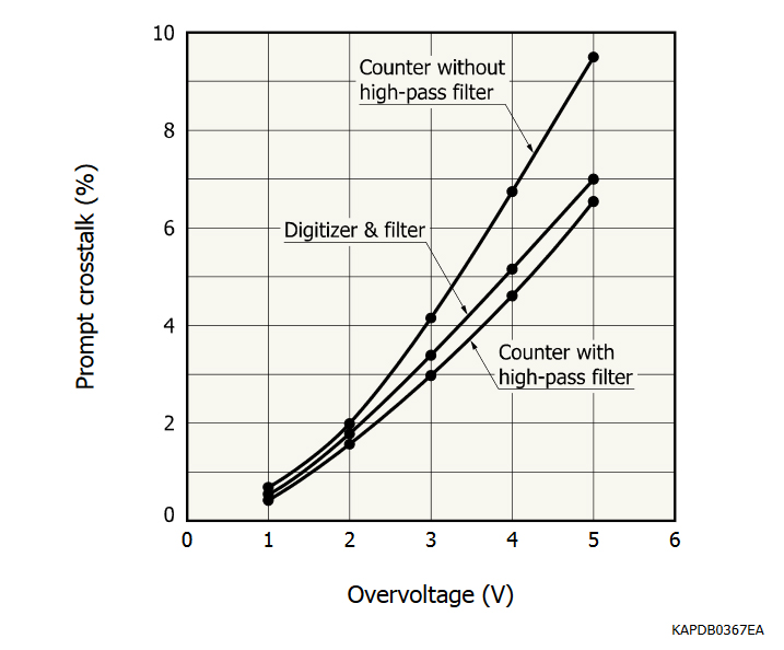
Figure 4-23 Prompt crosstalk vs. overvoltage
Figure 4-23: Prompt crosstalk comparison as measured by A. pulse counter with & without high-pass filter and B. digitizer. Use of a digitizer can cancel the effect of pulse pileup (as deduced from the linear slope) as would the use of a counter with high-pass filter.
Recovery time, afterpulse, and delayed crosstalk measurement: Figure 4-24 shows the flowchart of this measurement. In this case, we trigger the digitizer with MPPC output pulses. We then apply the filter to the output event, check whether the first pulse (used as trigger) has 1 p.e. pulse height, and reject the > 1 p.e. pulses because such pulses have differing probabilities of correlated noise pulses and hence disturb the following analysis. For the 1 p.e. pulse event, we then check arrival time and amplitude of next pulse and store the information into a memory array as part of this repetition loop.
The peak detection threshold after filtration should be as low as possible unless the remaining white noise reaches the threshold. In our example, we take the pulse height histogram of white noise output before beginning this loop, fit the histogram with Gaussian function, then take the 6σ value of the fitted function and use that value as the peak detection threshold.
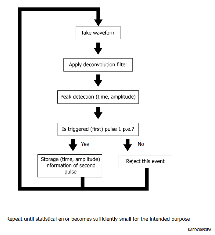
Figure 4-24 Flowchart of data-taking routine for our measurement program using digitizer and deconvolution
After data collection, we make a scatter plot of secondary pulses (arriving after the trigger pulse) in the manner shown in Figure 4-25 whose x-axis is the arrival time of a secondary pulse and y-axis is its amplitude. In practice, for verifying the measurement process’s progress, we have created a measurement software program to show this scatter plot whenever needed.
We now study the two event groupings circled by red and blue circles in Figure 4-25. The red group most likely consists of afterpulse events of the first (trigger) pulse considering that their pulse heights are less than 1 p.e. whereas the blue group consists of a combination of delayed crosstalk and accidental dark pulses that are not related to the first pulse considering that their heights are about 1 p.e.
We now isolate these groups from the scatter plot and analyze them separately to obtain the MPPC characteristics.
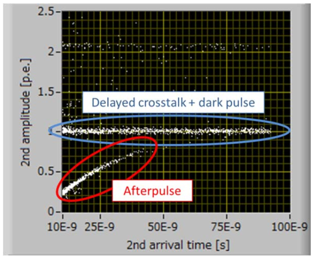
Figure 4-25 Scatter plot of timing and amplitude of secondary pulses
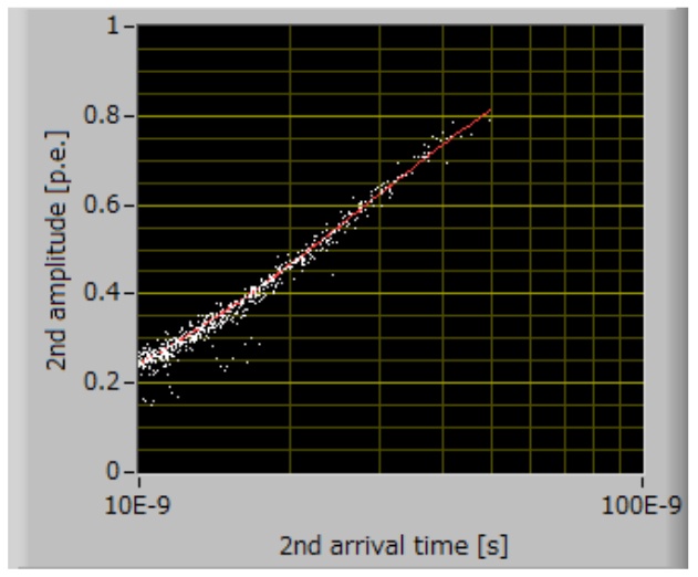
Figure 4-26 Trend line of afterpulse events of Figure 4-25 (circled in red)
- Recovery time analysis: Figure 4-26 shows the scatter plot of afterpulse events. From this, we can obtain the recovery time of this MPPC by fitting this plot to an exponential function and calculate its time constant. By this analysis, we obtain the recovery time of S13360-3050CS to be 30 ns.
The red line shows the exponential fitting of those events.
- Afterpulse analysis: Because of its nature, definition of the afterpulse probability is rather subjective due to the wide range of pulse heights and time delays that could constitute its definition. Thus, the concrete definition of MPPC afterpulse is dependent on the end-use application conditions and requirements. If the MPPC output current is read out continuously, all afterpulses and their charge contents will be integrated and included in the MPPC output current. On the other hand, when the MPPC output is read out as individual pulses, afterpulses whose pulse heights are lower than the counting discriminator threshold are ignored and would not be taken into account for assessing afterpulse probability; this means that measurement and quantification of afterpulse probability to a large extent depend on what lower-level discriminator threshold is used in the counting setup.
In the following, two definitions and analysis methods of afterpulse are showcased. The first definition simply sums the afterpulse events and calculates the percentage ratio of that sum to the total number of events. By this definition, afterpulse probability only counts the number of afterpulses whose pulse height exceeds the threshold level of the counter’s discriminator for pulse detection.
Hence, in specifying afterpulse probability based on this definition, the discriminator threshold level should be referenced.
An alternative but more complex definition utilizes a weighted integral of afterpulse events based on their pulse heights. Towards that, we first make a histogram of afterpulse events according to their arrival times (x-axis of Figure 4-26) as shown in Figure 4-27. Assuming that afterpulse probability has an exponential distribution, we fit this histogram to an exponential function to obtain the afterpulse probability distribution curve vs. arrival time. Afterwards, we calculate the product of this curve with the exponential function whose time constant corresponds to the recovery time (explained in preceding subsection) and proceed to compute the area under the resulting curve. Finally, we obtain the afterpulse probability as the ratio of this area to the total number of triggered events.
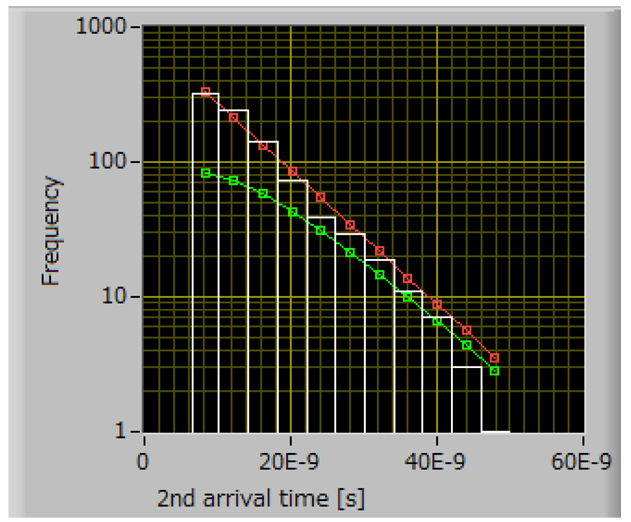
Figure 4-27 Histogram of afterpulse events
Note that compared to Figure 4-26, the y-axis now changes to frequency. The red line represents the exponential fitting of the histogram while the green line shows the product of afterpulse fitting and recovery time curve.
- Delayed crosstalk analysis: Figure 4-28 shows the histogram of the mixed events of delayed crosstalk and accidental dark pulses consisting of the events circled in blue in Figure 4-25. Different from afterpulse analysis, the resulting histogram does not appear as an exponential curve because it has two exponential components with different time constants.
To differentiate these, we have to fit this histogram to the sum of two exponential functions with different parameters. After a proper fitting is carried out, we can obtain the total number of delayed crosstalk events by calculating the area under the fitted exponential that corresponds to the delayed crosstalk component. Then, we can calculate the delayed crosstalk probability as the ratio of that area to the total number of triggered events.
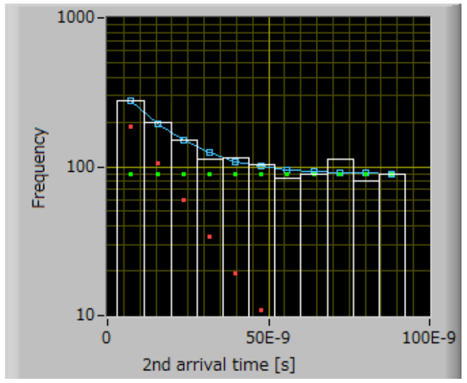
Figure 4-28 Histogram of mixed (delayed crosstalk and dark pulse) events. Red and green dots represent two exponential components.
- Measurement results: Figure 4-29 shows the probabilities of delayed crosstalk and afterpulsing of S13360-3050CS for various overvoltages.
Figure 4-29a Afterpulse and delayed crosstalk probabilities (S13360-3050CS)
(a) Afterpulse by counting vs. overvoltage
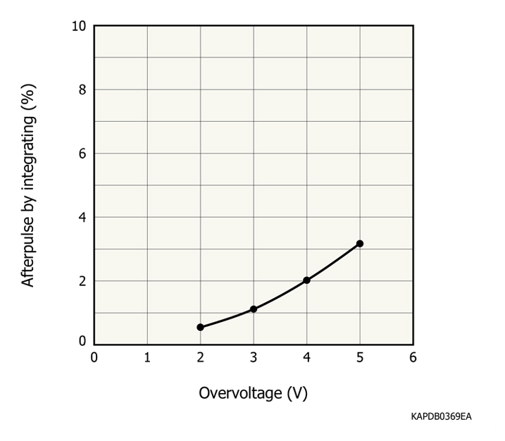
Figure 4-29b Afterpulse and delayed crosstalk probabilities (S13360-3050CS)
(b) Afterpulse by integrating vs. overvoltage
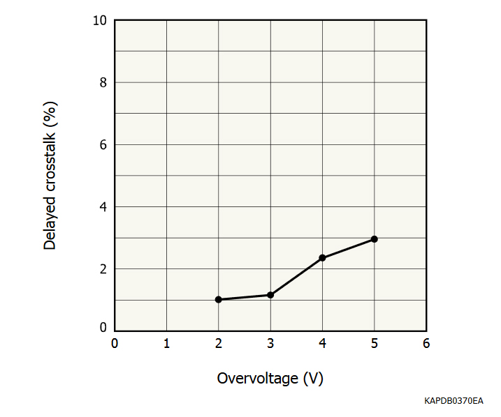
Figure 4-29c Afterpulse and delayed crosstalk probabilities (S13360-3050CS)
(c) Delayed crosstalk vs. overvoltage
4-6. Single-photon pulse shape measurement
- Measurement principle: Here we will explain how to take the single-photon/photoelectron (1 p.e.) waveform of the MPPC. The 1 p.e. waveform is essential to making the filter required for digital pulse processing and utilization of digitizer in MPPC characterization.
- Measurement setup: The setup for this measurement would be basically similar to that of measurements using a digitizer. One difference is that the bandwidth of each measurement setup component must be high enough to avoid degrading the high frequency component of MPPC output waveform. In this case, the maximum bandwidth of 1 GHz is sufficient for taking the 1 p.e. waveform of S13360-3050CS. Another difference is that the min. data collection time window would be set by the full width of the 1 p.e. waveform. In this case of S13360-3050CS, a time window of 200 ns would be adequate.
- Measurement procedure: We obtain the MPPC’s output waveform. Then, after checking the number of pulses in the waveform and their heights, we decide whether the triggered pulse is a genuine 1 p.e. waveform or not (i.e. prompt/delayed crosstalk or afterpulse following a dark pulse) and store an output pulse only when it is confirmed to have a 1 p.e. waveform. Afterwards, this step must be repeated a sufficient number of times to ensure the elimination of white noise by averaging all stored 1 p.e. waveforms.
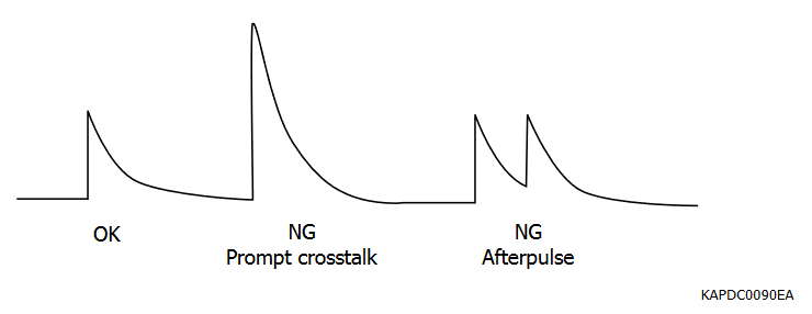
Figure 4-30 “Genuine” 1 p.e. waveform of dark pulse. Others should be excluded from 1 p.e. waveform storage and accumulation.
- Measurement result: Figure 4-31 shows the result of measuring the 1 p.e. waveform of S13360-3050CS.
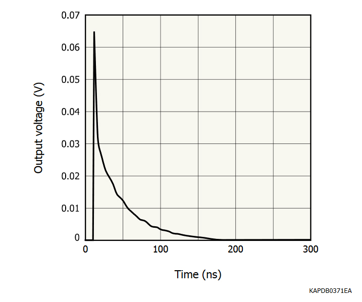
Figure 4-31 1 p.e. waveform (S13360-3050CS)
4-7. Time resolution ability
Photodetector time resolution characteristics are critical to attaining proper performance in direct-TOF (time-of-flight) applications such as TOF-PET (positron emission tomography) in medical imaging or LiDAR (light detection and ranging) in 3D scanning to determine the arrival times of signal photons or radiation. In this subsection, we will describe measuring two particularly-relevant time resolution characteristics: coincidence time resolution (CTR) and single photon time resolution (SPTR).
-CTR:
- Measurement principle: In TOF-PET, CTR is measured by using two detector channels, each consisting of a pair of scintillator crystal and photodetector, to detect gamma rays, having 511 keV in energy, that are emitted simultaneously from a positron decay and the resulting electron-positron annihilation.
The measurement setup is shown in Figure 4-32. The detection times obtained from detector channels 1 and 2 should ideally show the same value if each detector has the same distance from the radiation source as the other. However, variations in underlying factors such as the scintillator’s light emission yield, the photodetector’s internal charge collection efficiency, photon detection efficiency, and output pulse shape, and the output amplifier’s characteristics cause some timing variation between the two detector channels. The probability distribution curve of the timing difference between detector channels 1 and 2 has a bell-shaped Gaussian-like profile. CTR is theoretically defined by the FWHM of this distribution profile.
The result of this measurement does not represent the time resolution of the photodetector (i.e. MPPC) itself but the overall system time resolution, including the scintillator, amplifier, trigger circuitry, and other instruments utilized besides the photodetector.
- Measurement setup:
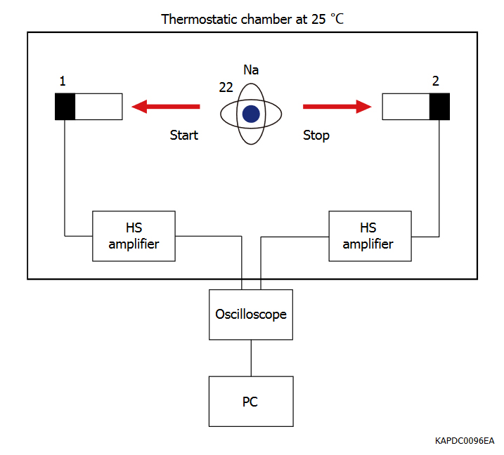
Figure 4-32 CTR (coincidence resolving time) measurement setup
Equipment:
Radiation source: Na-22, etc.
Scintillator: LFS, LSO, LYSO, etc.
Amplifier: linear amplifier (internal product and not for sale), bandwidth: 1 GHz
Oscilloscope: SDA 760Zi (LeCroy)
Procedure:
The radioisotope should be positioned in the middle of detectors to equalize its distance from them. Originating from the annihilation of the positron byproduct of Na-22’s radioactive decay, gamma rays (if emitted in the proper opposite directions) reach detector channels 1 and 2 at the same time. The gamma rays undergo scintillation once detected, with the emitted scintillation light in turn detected by each photodetector (i.e. MPPCs). Generally speaking, CTR measurement is limited by the system’s timing jitter. To measure CTR with a specific target time jitter, the utilized output amplifier circuitry must have sufficient bandwidth to allow the jitter’s proper detection.
The amplified output pulses are then read out by a high-speed oscilloscope. The oscilloscope can calculate the time differences between coincident pairs of pulses outputted by the two detector channels, can profile the distribution of those differences (as obtained from a sufficiently-large population of such coincident pulses), and then produce the FWHM of that distribution in order to determine the measured CTR. The utilized oscilloscope should also have adequately wide input bandwidth and high sampling rate in order to resolve picosecond timing. One can also use a combination of TAC and MCA instead of a wide-bandwidth high-speed oscilloscope.
Figure 4-33 shows the linear output amplifier’s output pulse shape coming from two Hamamatsu S13360 series MPPCs. The key to high-accuracy measurement results is to decrease baseline fluctuations as much as possible. The optimal way to do so would depend on the measurement setup and the target application, but would consist of controlling the trigger threshold level, the bias voltage applied to the MPPC, and the measurement’s optical conditions amongst other factors.
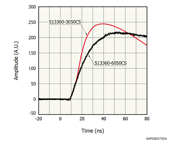
Figure 4-33 Output pulse from linear output amplifier
- SPTR:
- Measurement principle: SPTR is a parameter that characterizes the MPPC’s time resolution alone; this is in contrast to CTR, which evaluates a system’s overall time resolution performance. The basic idea of this measurement is to illuminate the MPPC with a single-photon input signal light level and to then determine the detection times of single photons by recording the MPPC’s output pulses (using a 1 p.e. trigger threshold level). The measurement setup is shown in Figure 4-34.
The suitable light source for this measurement would be able to produce light pulses of picosecond width; Hamamatsu’s PLP-10 would be one such light source.
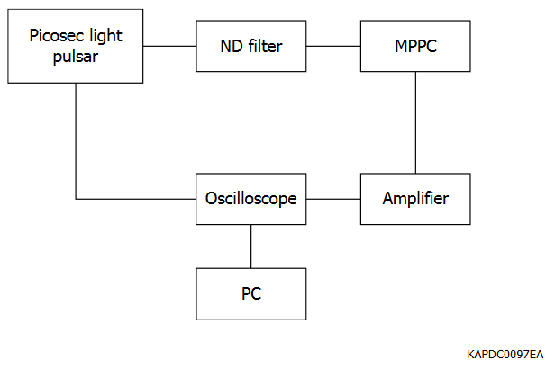
Figure 4-34 SPTR measurement setup
Equipment:
Light source: PLP-10 (Hamamatsu Photonics K.K.)
ND filters
Amplifier: linear amplifier (internal product and not for sale), bandwidth: 1 GHz
Oscilloscope: SDA 760Zi (LeCroy)
Procedure: The basic measurement method is the same as CTR except that SPTR measurement relies on an output pulse height of only 1 p.e. Once a light intensity that results in majority 1 p.e. output pulses is attained, pulse heights greater than 2 p.e. and lower than 1 p.e., which would correspond to crosstalk and afterpulsing, must be excluded by using upper- and lower-level discriminator thresholds set at 1.5 p.e. and 0.5 p.e. levels. This measurement requires careful cabling to minimize parasitic noise as SPTR is easily affected by baseline deteriorations.
The variation of the timing information obtained by this method includes not only MPPC’s pulse time jitter but also the light source’s pulse emitting jitter. Thus, MPPC’s SPTR is derived as:
Equation 4-1
4-8. Dynamic range and linearity measurement
As discussed in Section 2, MPPC’s linearity is limited by its PDE, pixel count per unit of area, and recovery time. In this subsection, we will describe a generalized measurement method to estimate the MPPC’s pulse-rate linearity.
- Measurement principle: Before we discuss the measurement procedure, let’s recall two key aspects of MPPC linearity and dynamic range from Section 1: First, a MPPC pixel cannot distinguish the number of simultaneously-incident photons upon it; the pixel response is limited to outputting a 1 p.e. pulse whose height does not depend on the number of incident photons. Second, each pixel requires a certain duration of recovery time. A photon’s incidence onto a pixel after a preceding photon’s detection cannot cause a full-height secondary output signal within the recovery time.
The first aspect (assuming we’re restricted to a fixed pixel size to maintain PDE) can be alleviated by dispersing the input light signal (using a diverging lens or by other means) to decrease the number of incident photons per unit area onto the MPPC. However, both aspects can be addressed by using a MPPC of smaller pixel size; such a MPPC would have an increased count of pixels per unit of area (i.e. more pixels within the same optical field-of-view) available to detect incident photons and a decreased pixel recovery time due to lower pixel capacitance. However, these advantages have a tradeoff of loss in PDE due to the lower fill-factor of a smaller pixel; thus, the lower limit of the linearity of such a MPPC is shifted upwards.
In order to measure MPPC linearity, we use the photon counting technique for the lower levels of the MPPC’s linearity where the signal level intensities are low and the current measurement technique (similar to measuring I/V curve) for the upper levels of MPPC’s linearity. In this measurement, we use a DC light source for implementing both techniques; we control the light level using an optical attenuator and ND filters. A key issue is accurate determination of the light intensity that the MPPC has detected at each obtained data point. This is accomplished by precise monitoring of the incident light intensity using a calibrated monitor photodiode. A peculiar aspect of doing so is in the photon-counting regime: the light intensity incident on the MPPC is adjusted to reach that regime using a precise ND filter while the calibrated photodiode can monitor the total (pre-attenuation) light intensity present with high accuracy.
- Measurement setup:
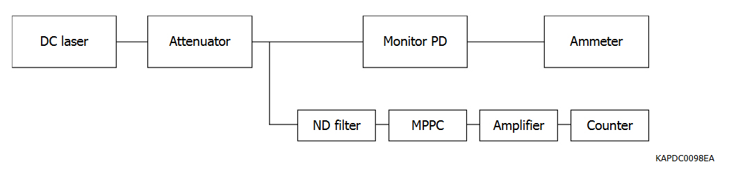
Figure 4-35 Measurement setup (Low intensity light level)
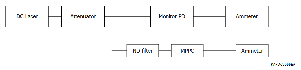
Figure 4-36 Measurement setup (High intensity light level)
Equipment:
Light source: CW laser
Optical attenuator
ND filter
Amplifier: linear amplifier (internal product and not for sale), Bandwidth: 1 GHz
Counter: 53131A (Agilent)
Procedure:
We first measure and calibrate the ND filter’s attenuation rate using the calibrated photodiode. We recommend an ND filter that has 2-3 orders of magnitude attenuation capability. In the following measurement, the attenuation rate obtained here is used to estimate the light intensity incident onto the MPPC. One can adjust that light intensity over the MPPC’s full dynamic range (from photon counting to saturation) by controlling the optical attenuator.
Low intensity light level
While the light intensity on the MPPC is at the photon-counting level, one can measure the MPPC’s output response linearity by gradually increasing the light level. This task is similar to measuring dark counts but with the lower-level discriminator’s threshold set to be 0.5 p.e. Here, we define “photon counting level” to be a light intensity that results in MPPC output pulse heights of only 1 p.e. with enough inter-pulse time interval for continual detection of individual incident photons. Figure 4-35 shows the corresponding setup.
High intensity light level
We switch to the current measurement technique once the light intensity becomes high enough to result in the occurrence of ≥ 2 p.e. output pulse heights in order to avoid counting errors due to pulse pileup. Figure 4-36 shows the corresponding setup. In this measurement, the MPPC’s output current is measured using an ammeter, which is then followed by subtraction of dark current in order to obtain the net photon-correlated current. As increases in incident light intensity continue, one will eventually see the output’s saturation.
The combined linearity plot (of low and high input light intensities) is obtained by using the pulse count rate of the low-intensity measurement (by dividing the integrated count of detected 1 p.e. pulses at each data point by the integration time used for measuring each data point) and of the high-intensity measurement (by dividing the measured net (dark-subtracted) current by the charge output corresponding to a 1 p.e. pulse).
Figure 4-37 is the measured linearity plot of a Hamamatsu MPPC with a 15 μm pixel pitch. In this plot, the light level is indicated as number of incident photons per unit of time (in counts per second or cps).
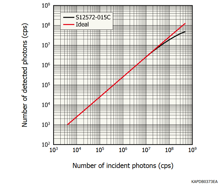
Figure 4-37 Measurement result of dynamic range (S12572-015C)
References
Section 1
[1] Donald A. Neamen, Semiconductor Physics and Devices, 3rd ed. New York, NY: McGraw-Hill, 2003.
[2] Ben G. Streetman, Solid State Electronic Devices, 3rd ed. Englewood Cliffs, NJ: Prentice Hall, 1990.
[3] John Gowar, Optical Communication Systems, London, UK: Prentice Hall Intl. Ltd., 1984.
[4] Silvano Donati, Photodetectors: Devices, Circuits, and Applications, Upper Saddle River, NJ: Prentice Hall, 2000.
[5] S. M. Sze, Physics of Semiconductor Devices, 2nd ed. New York, NY: John Wiley & Sons, 1981.
[6] D. Renker and E. Lorenz, “Advances in Solid State Photon Detectors,” Journal of Instrumentation, volume 04, issue 04, pp. 04004, April, 2009.
Section 2
[7] James W. Nilsson, Susan A. Reidel, Electric Circuits, 6th ed. Englewood Cliffs, NJ: Prentice Hall, 2000.
[8] Tudor E. Jenkins, Optical Sensing Techniques and Signal Processing, London, UK: Prentice Hall Intl. Ltd., 1987.
[9] M. Grodzicka, et al. “MPPC Array in the Readout of CsI:Tl, LSO:Ce:Ca, LaBr:Ce, and BGO Scintillators,” IEEE Trans. Nucl. Sci., vol. 59, no. 6, Dec. 2012.
[10] Helmuth Spieler, “Fast Timing Methods for Semiconductor Detector,” IEEE Trans. Nucl. Sci., vol. NS-29, no. 3, pp. 1143-1158, June, 1982.
Section 4
[11] P. Eckert, et al. (2010, April 1). Characterization Studies of Silicon Photomultipliers (2nd ed.) [Online]. Available: https://arxiv.org/abs/1003.6071
[12] Steven W. Smith, The Scientist & Engineer's Guide to Digital Signal Processing, San Diego, CA: California Technical Publishing, 1997.
[13] H. Oide, “半導体光検出器 PPD の基本特性の解明と,実践的開発に向けた研究,” M.S. thesis in Japanese, 2009. [Online]. Available: https://www.icepp.s.u-tokyo.ac.jp/papers/ps/thesis/master/oide_mthesis.pdf [66KB/PDF]
[14] Adam N. Otte, et al. (2016, June 16). Characterization of Three High Efficiency and Blue Sensitive Silicon Photomultipliers [Online]. Available: https://arxiv.org/abs/1606.05186
[15] J. Rosado, S. Hidalgo. (2015, Oct. 21). Characterization and Modeling of Crosstalk and Afterpulsing in Hamamatsu Silicon Photomultipliers (2nd ed.) [Online]. Available: https://arxiv.org/abs/1509.02286
- Confirmation
-
It looks like you're in the . If this is not your location, please select the correct region or country below.
You're headed to Hamamatsu Photonics website for US (English). If you want to view an other country's site, the optimized information will be provided by selecting options below.
In order to use this website comfortably, we use cookies. For cookie details please see our cookie policy.
- Cookie Policy
-
This website or its third-party tools use cookies, which are necessary to its functioning and required to achieve the purposes illustrated in this cookie policy. By closing the cookie warning banner, scrolling the page, clicking a link or continuing to browse otherwise, you agree to the use of cookies.
Hamamatsu uses cookies in order to enhance your experience on our website and ensure that our website functions.
You can visit this page at any time to learn more about cookies, get the most up to date information on how we use cookies and manage your cookie settings. We will not use cookies for any purpose other than the ones stated, but please note that we reserve the right to update our cookies.
1. What are cookies?
For modern websites to work according to visitor’s expectations, they need to collect certain basic information about visitors. To do this, a site will create small text files which are placed on visitor’s devices (computer or mobile) - these files are known as cookies when you access a website. Cookies are used in order to make websites function and work efficiently. Cookies are uniquely assigned to each visitor and can only be read by a web server in the domain that issued the cookie to the visitor. Cookies cannot be used to run programs or deliver viruses to a visitor’s device.
Cookies do various jobs which make the visitor’s experience of the internet much smoother and more interactive. For instance, cookies are used to remember the visitor’s preferences on sites they visit often, to remember language preference and to help navigate between pages more efficiently. Much, though not all, of the data collected is anonymous, though some of it is designed to detect browsing patterns and approximate geographical location to improve the visitor experience.
Certain type of cookies may require the data subject’s consent before storing them on the computer.
2. What are the different types of cookies?
This website uses two types of cookies:
- First party cookies. For our website, the first party cookies are controlled and maintained by Hamamatsu. No other parties have access to these cookies.
- Third party cookies. These cookies are implemented by organizations outside Hamamatsu. We do not have access to the data in these cookies, but we use these cookies to improve the overall website experience.
3. How do we use cookies?
This website uses cookies for following purposes:
- Certain cookies are necessary for our website to function. These are strictly necessary cookies and are required to enable website access, support navigation or provide relevant content. These cookies direct you to the correct region or country, and support security and ecommerce. Strictly necessary cookies also enforce your privacy preferences. Without these strictly necessary cookies, much of our website will not function.
- Analytics cookies are used to track website usage. This data enables us to improve our website usability, performance and website administration. In our analytics cookies, we do not store any personal identifying information.
- Functionality cookies. These are used to recognize you when you return to our website. This enables us to personalize our content for you, greet you by name and remember your preferences (for example, your choice of language or region).
- These cookies record your visit to our website, the pages you have visited and the links you have followed. We will use this information to make our website and the advertising displayed on it more relevant to your interests. We may also share this information with third parties for this purpose.
Cookies help us help you. Through the use of cookies, we learn what is important to our visitors and we develop and enhance website content and functionality to support your experience. Much of our website can be accessed if cookies are disabled, however certain website functions may not work. And, we believe your current and future visits will be enhanced if cookies are enabled.
4. Which cookies do we use?
There are two ways to manage cookie preferences.
- You can set your cookie preferences on your device or in your browser.
- You can set your cookie preferences at the website level.
If you don’t want to receive cookies, you can modify your browser so that it notifies you when cookies are sent to it or you can refuse cookies altogether. You can also delete cookies that have already been set.
If you wish to restrict or block web browser cookies which are set on your device then you can do this through your browser settings; the Help function within your browser should tell you how. Alternatively, you may wish to visit www.aboutcookies.org, which contains comprehensive information on how to do this on a wide variety of desktop browsers.
5. What are Internet tags and how do we use them with cookies?
Occasionally, we may use internet tags (also known as action tags, single-pixel GIFs, clear GIFs, invisible GIFs and 1-by-1 GIFs) at this site and may deploy these tags/cookies through a third-party advertising partner or a web analytical service partner which may be located and store the respective information (including your IP-address) in a foreign country. These tags/cookies are placed on both online advertisements that bring users to this site and on different pages of this site. We use this technology to measure the visitors' responses to our sites and the effectiveness of our advertising campaigns (including how many times a page is opened and which information is consulted) as well as to evaluate your use of this website. The third-party partner or the web analytical service partner may be able to collect data about visitors to our and other sites because of these internet tags/cookies, may compose reports regarding the website’s activity for us and may provide further services which are related to the use of the website and the internet. They may provide such information to other parties if there is a legal requirement that they do so, or if they hire the other parties to process information on their behalf.
If you would like more information about web tags and cookies associated with on-line advertising or to opt-out of third-party collection of this information, please visit the Network Advertising Initiative website http://www.networkadvertising.org.
6. Analytics and Advertisement Cookies
We use third-party cookies (such as Google Analytics) to track visitors on our website, to get reports about how visitors use the website and to inform, optimize and serve ads based on someone's past visits to our website.
You may opt-out of Google Analytics cookies by the websites provided by Google:
https://tools.google.com/dlpage/gaoptout?hl=en
As provided in this Privacy Policy (Article 5), you can learn more about opt-out cookies by the website provided by Network Advertising Initiative:
http://www.networkadvertising.org
We inform you that in such case you will not be able to wholly use all functions of our website.
Close