Application notes


Technical notes
Ask an engineer


Publications
United States (EN)
Select your region or country.
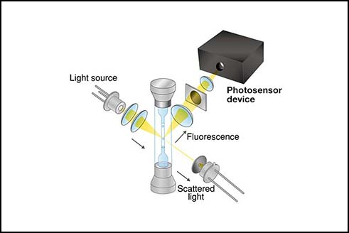
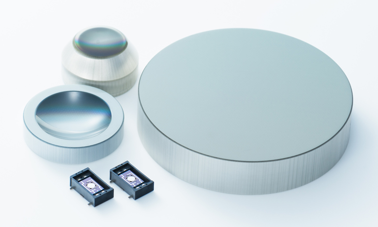
Head-on PMT product selection
Ardavan Ghassemi, Hamamatsu Corporation
January 11, 2018
Table of Contents
In this technical note, an overview of generalized methods for selection of head-on PMT products for a broad range of applications is provided.
A primary objective has been to describe methods that could be used for any application as long as certain basic pieces of information are available about the target application; these methods could be used for product selection consistently despite the application’s peculiarities.
However, it is important to note that the methods described in this technical note are meant to serve as preliminary general guidelines (so-called ‘back-of-the-envelope’ calculations); they are intended to serve as early indicators of what product(s) to begin considering for evaluation. As the technical considerations advance, these methods would not substitute proper simulation and experimentation under the specific conditions of the intended application.
The content of this technical note assumes a working knowledge of characteristics and operation principles of PMTs. For more information on those topics, please refer to Hamamatsu’s General PMT Catalog, HEP PMT Catalog, and Photomultiplier Tube Handbook. This technical note consists of two main sections; the first section provides an overview of methods to assess photodetector performance, and the second describes how to put those methods to use.
Section 1. PMT performance parameters
Each and every application that involves detection of light (regardless of its source: laser, LED, lamp, scintillation, different luminescence effects, etc.) can be defined and characterized by the following parameters:
1.1 Signal
An optical application's input signal level is simply the amount of light that is to be detected. The input light signal has a spectral distribution, which is typically represented in simplistic calculations (such as the methods to be described here) by the peak wavelength. In quantifying the amount of input signal present, suitability of the dimension or unit of measurement is essential for making proper calculations.
Two common dimensions that could be used by the methods described in this technical note are watts [W] and number of photons. Note that the former is normalized to time while the latter is not (although the latter could be, and both can be normalized to illumination area). A signal level expressed in either of these units can be converted to the other by the following formula:
Eq. 1.1a
Where:
T = illumination time for a measurement
There are other units (lm, lx, etc.) used to express the amount of light present, but those units require tabulated reference data or complex calculations for their proper use, and hence, they are not discussed in this technical note as they exceed its intended scope.
Input light signal can be converted to output signal of a photodetector by the following relationship:
Eq. 1.1b
Where:
Sdark = the detector output charge that is not generated as a result of the photoelectric effect during the measurement
CE = collection efficiency
M = multiplication gain
Often, photon detection efficiency or PDE is used by customers as defined by PDE = QE x CE. It is also noteworthy to mention that Hamamatsu's PMT gain specification is in fact CE x M; however, users typically account for these two parameters separately.
1.2 Noise
The intrinsic uncertainty or random fluctuation in a measured signal is noise.
For an optical signal, that uncertainty or noise is characterized through a histogram (a so-called pulse height distribution or PHD) of incidents of detected light pulses with varying heights (i.e., containing different counts of photons); the resulting histogram could be closely fitted into a profile similar to that of a Poisson probability distribution.
That leads us to conclude that noise characteristics of a photon signal can be modeled by the following Poisson probability distribution function and its corresponding mean (μ) and standard deviation (σ):
Eq. 1.2a
To model the detection of light using the above probability model, the standard deviation is considered a measure of randomness or uncertainty (i.e., noise) of the Poisson random variable (i.e., photon signal), and the mean is the expected value of the signal.
In other words, intrinsic noise of a light signal is described by the square root of its mean. A photodetector's dark output also has a Poisson probability distribution.
A noise whose random behavior can be characterized by a Poisson distribution is often referred to as "shot" noise.
1.3 Signal-to-noise ratio (SNR)
As its name suggests, it is the ratio of signal to noise as calculated for a detector's output. In light detection applications with unity gain, it's fundamentally defined by:
Eq. 1.3a
Where:
nphoton shot = photon shot noise
ndark shot = dark shot noise
nreadout = readout noise at the applicable sampling frequency
However, since readout noise can typically be ignored because of a PMT's high gain, more practically and for the analog mode of PMT operation, the following equation can be used:
Eq. 1.3b
Where:
F = excess noise factor (F ~ 1.2 for a typical PMT)
q = the fundamental charge
Δf = readout amplifier bandwidth
Φ = QE ⋅ λ / 124000 - the PMT's radiant photosensitivity [A/W] in whose calculation QE is a percentage and λ is wavelength [nm]
In Eq. 1.3b, Sinput is in the unit of W and Ik_dark as photocathode dark current is in the unit of A.
In photon counting, considering the binary nature of the readout scheme in photon counting, readout noise is forgone, and the following equation (see Note 1) would be used per measurement reading:
Eq. 1.3c
Where:
Nphoton = the number of photons incident onto the PMT
(Nphoton x PDE) = the number of photoelectrons detected
Ndark = the PMT's dark (~1p.e. in height under no illumination) output pulse count during a measurement
The latter portion of Eq. 1.3c is particularly useful in experimental determination of photon-counting SNR with Ntotal being obtained from dividing the PMT's total output charge by the amount of output charge corresponding to 1p.e. pulse height; these counts (Ntotal and Ndark) would be calculated by performing PHD analysis on the integrated PMT output pulse data.
Note 1:
The derivation of the denominator of Eq. 1.3c’s second half is often a point of curiosity. If we define (T – D) as a random variable to be the photo-signal (i.e., Dark-subtracted Total output signal measured under illumination), then its variance would be:
Since total output signal and dark signal are uncorrelated, we have:
Thus, RMS combination of shot noises of dark signal and photo-signal becomes:
Bear in mind that Eq. 1.3a-c assume that the signal to be measured is the only light flux incident on the detector (i.e., no background light).
1.4 Linearity
The extent to which a photodetector's output has a linear relationship with its input (as defined by f(x) = b⋅x + c in which b and c are real constants) is the measure of the photodetector's linearity and is fundamentally defined by:
Eq. 1.4a
in which A is signal amplitude and t represents passage of time. If the ratio of the 2 relative changes is < 1, nonlinearity exists. For practical purposes, nonlinearity is typically of greater interest than linearity itself:
Eq. 1.4b
Since photodetector response is theoretically linear (within the constraints of SNR > 1 and up to saturation), linearity can be practically obtained by:
Eq. 1.4c
In terms of detector response, there are 3 particular definitions of linearity: DC linearity, pulse rate linearity, and pulse rate and detector bandwidth.
DC linearity
This is a measure of how mean output of a detector changes linearly with respect to changes in average light input over a period of time. Understanding the concept of ‘DC’ linearity within the context of an average over a single measurement’s time duration is important: linearity can be feasibly assessed by relying on data points of mean response (integrated during each measurement reading and thus averaged per its time duration) for signals with randomly fluctuating amplitudes or non-harmonic repetitions.
Pulse height linearity
This is the relative extent by which a change in an input light pulse’s amplitude results in a change in the photodetector’s output pulse.
Pulse rate and detector bandwidth
This is a measure of a photodetector’s pulse height behavior as a function of input signal frequency. Ideally, there must be no dependence; however, in practice, an undesirable effect known as ‘pulse pileup’ occurs with output pulse heights (i.e., signal level difference between peaks and valleys of pulses) decreasing as frequency increases to exceedingly higher levels.
For fixed readout impedance, pulse rate characteristic is limited by a detector’s electrode design, internal capacitance and inductance.
For a pulsed input signal of fixed amplitude but increasing frequency, bandwidth is defined as the frequency [Hz] at which amplitudes of output pulses decline by a certain amount compared to a DC input signal of the same amplitude.
Bandwidth is a concern in the design of output amplifier circuits and other readout electronics, considering that a larger amplifier bandwidth allows the passage of a wider spectrum of noise frequency components to the output while bandwidth must be larger than the highest-frequency component of the input light in order to allow its proper detection. Thus, the designer of a detector system seeks to select a detector with a cutoff frequency that is by a conservative margin above the highest-frequency component of the signal and then design a readout amplifier circuit whose bandwidth is also by a conservative margin above the highest-frequency component of the signal.
In a pulsed application, if the study of individual light pulses is intended for instance, the signal’s highest-frequency component is the product of the constant 0.35 and the inverse of the shortest pulse rise or fall time (10% to 90% or vice versa of amplitude) that is to be measured. Furthermore, the readout amplifier circuit’s cutoff frequency at -3dB should be designed to be at least twice that of the signal’s highest-frequency component whose measurement is desirable (but as a general rule of thumb, 4 times is an advisable design target).
1.5 Dynamic range
Dynamic range (DR) is typically expressed as a ratio between two levels of the input signal. One level (as numerator of the ratio) is the highest amount of input signal at which the detector maintains its response linearity (i.e., nonlinearity < application's requirement). The other (denominator of the ratio) is the lowest amount of input signal at which the detector behaves linearly.
Over a detector's DR, nonlinearity at the lower limit is typically limited by noise (whether dark or readout noise or a combination thereof), or in other words, the amount of input signal that yields SNR = 1 (often measured and divided by square root of the bandwidth and then specified as noise-equivalent power ).
On the other hand, nonlinearity at DR's upper limit is typically caused by saturation effects. In a PMT's case, the saturation effect differs between DC and pulsed operations. In DC operation, upper linearity is limited by how much current the PMT's voltage divider can supply to its dynodes.
In pulsed operation, upper linearity is limited by space-charge effects (i.e., charge density of a preceding electron cloud repelling a succeeding one and hampering its progression) amongst the later dynode stages.
1.6 Time response
As represented by a photodetector's rise and fall times, this is an indicator of how closely the output of a photodetector temporally resembles the shape of its input.
It is particularly important for applications in which maintaining the pulse shape integrity of the input signal is desirable for pulse shape discrimination (PSD); in those cases, the detector's rise and fall times must be shorter than rise/fall times of input light pulses. For a fixed readout scheme, a detector's time response (rise/fall times) is proportional to its capacitance.
1.7 Time resolution
The limiting uncertainty that exists in determining the timing of a detected event with respect to a reference point in time (which could be another detected event) is called time resolution. In optical applications, that is the overall uncertainty in timing the detection of input light pulses and is fundamentally defined by:
Eq. 1.7a
In this formula, pulse timing is that aspect of a detected pulse that is used for determining the time of its detection. For example, if the time measurement system is edge-triggered, timing will be a portion of the rise time of the pulse (depending on the trigger's set threshold).
On the other hand, if level-triggered, timing would be the time duration of that portion of the pulse shape that defines level. In how the photodetector output signal is amplified and used for triggering, fluctuations in the formation of this timing parameter (called amplitude time walk) cause a variance in measuring time.
Additionally, time stamping is the recording of the signal's timing by the measurement system once the trigger requirement has been met. This parameter also experiences a variance (typically due to digitization noise in conventional measurement systems).
However, since caused by the photodetector alone and as the limiting factor in the overall time resolution of a light detection system, detector jitter is the parameter of interest to our discussion.
Considering the Poisson nature of photoelectron signal and noise, we can conclude that the jitter is proportional to the inverse of the square root of the number of photoelectrons:
Eq. 1.7b
This relationship provides a highly effective tool in preliminary technical discussions with customers, but one must understand its limitation: it is only applicable to timing at point of charge generation and excludes any variability in delays that might be present in charge collection and readout.
1.8 Measurement
Sometimes referred to by other terms such as a data point, a sampling, a reading, or an event, a measurement is a single experimental attempt [temporally (per a duration of time) and spatially (per a detector channel and within its physical size and field-of-view)] to quantify an optical signal.
The result of a measurement is thus a piece of quantitative data that represents essential information about the true signal. Measurement is a very fundamental and seemingly simple concept, so why is it explored here?
There are 3 important points to keep in mind:
Measurement frequency
Understanding the required bandwidth for a measurement is of paramount importance to proper identification and definition of an application's requirements and in order to compare those requirements with characteristics of candidate photodetectors.
Fundamentally, based on Nyquist's sampling theorem, the sampling frequency must be at least twice the measurement frequency, which in turn would be equal to the frequency of the signal's highest-frequency component that is intended to be detected.
Furthermore, as discussed before, a readout amplifier circuit's cutoff frequency at -3dB should be designed to be at least twice that of the measurement frequency (but as a general rule of thumb, 4 times is an advisable design target).
For better illustration, the following examples portray cases in which a detrimental bandwidth mismatch is present:
- Using an amplifier with a cutoff frequency of 1MHz to measure pulses with frequency of 900kHz and rise/fall times of ~1μs
- Using an imager with a spatial resolution of 10lp/mm to contact-image a min. feature size of 20μm. [Reason: 10lp/mm is theoretically able to observe a min. feature size of 1mm /(2 x 10) = 50μm]
- Using an oscilloscope with a sampling rate of 150MHz to look for multiple randomly occurring events with durations of 10ns each. (Reason: 150M < 2 x 1/10n = 200M)
Measurement resolution and range
Besides measurement frequency, the resolution of the measurement instrumentation in its ability to accurately resolve the smallest expected quantity of or change in the parameter (that is to be measured) over the full range of its expected values is also of great importance.
The following are examples in which there is a detrimental mismatch between signal characteristics and measurement resolution and range:
- Using an 8-bit digitizer with a conversion factor of 500Ke-/LSB to plot pulse height distribution for up to 150 p.e. pulses of a PMT at gain = 1E6. (Reason: 150 x 1E6/5E5 = 300 > 28)
- Using a detector with a rise time of 10ns to discriminate the pulse shapes of 2 signals with rise times of 1ns and 8.5ns.
- Using a spectrometer with a resolution of 30nm to distinguish emission or excitation peaks 10nm apart.
- Using a 16-bit/sample ADC with a bit rate of 50Mbps to record the output waveform of an MPPC with a dark count rate of 4Mcps for under dark conditions. (Reason: 50M / 16 < 4M)
Normalizations
While some signal characteristics (like amplitude, timing or frequency) can be appropriately obtained from measuring a single parameter (whether once or a multitude of times), others (like flux or power) would by definition include normalizations to time and/or spatial information and hence require measurements of 2 or more parameters in order to be quantified.
These differences are important, since a typical instrument designer is naturally concerned with the performance of her overall instrumentation: she could be designing for an application condition that combines a series of measurements and contains one or more normalizations instead of consisting of a single parameter alone.
In order to assess a photodetector's suitability for a given application, one must bear that in mind and see how the way detector characteristics have been specified compares with the designer's presumed application conditions and target requirements.
Towards that, one would begin by finding out to what temporal or spatial parameters a stated application condition might have been normalized; when in doubt, one should make sure about the dimension or unit of the application condition in question. Furthermore, it is also important to understand the scope of those normalizations. For example, one needs to examine whether the incident light "power" is applied to the entirety of a detector's active area or normalized to pixel count or unit of area.
As another example, it is important to verify whether peak power or average power is meant when a reference to incident light "power" is made; peak and average power have different temporal normalizations in that the former is the ratio of energy content of a single pulse to the time duration of that pulse while the latter takes the time in between consecutive pulses into account. As a further example, if various spectral band components of a broad spectrum of light are to be detected by different detector channels separately (applicable to 1D or 2D serial- or parallel-readout multichannel detectors), performance of each detector channel must be assessed independently in accordance to its particular expected input light signal conditions.
Section 2. Case studies of assessing PMT performance
In this section, we will conduct a study of PMT product selection calculations. As part of this review, we will learn a number of key techniques to perform such calculations.
As described earlier, please keep in mind that optical power [W] or electric current [A], whose dimensions are normalized to time, can be converted to units of photons or electrons per second (and vice versa) using Eq. 1.1a or the fundamental charge conversion constant (1.6E-19C/e-).
Now, let's suppose that a customer has the following application conditions:
- Peak wavelength of ~420nm
- 1 to 1E4 photons per pulse
- Pulse rates of 1k-1MHz
- Typical pulses having widths of ~8ns and decay times of ~5ns
And with the following requirements: absolute intensity of each pulse must be measured with nonlinearity below 5%, and a time resolution of 70ps must be attained for pulses larger than 100 photons. Furthermore, the customer's design allows for a 1" dia. detector active area or field-of-view (FOV).
Note that the application conditions are fairly generic; many seemingly important details, such as what source is producing the light signal, don't affect these back-of-the-envelope calculations.
2.1 SNR
To begin, we rely on the following generalized assumptions about a typical PMT's characteristics: QE of 25% at 420nm for a bialkali photocathode, CE of 0.85, and gain (see Note 2) of 1E6. As the discussion progresses, these assumptions must be revisited and either verified or revised.
Note 2: However, please note that gain values listed in Hamamatsu's PMT catalog include CE. This is because PMT gain is calculated by dividing anode sensitivity by cathode sensitivity; anode sensitivity already includes the factor of CE.
Using Eq. 1.1b, we calculate a hypothetical PMT's charge output per pulse:
For 1 photon per pulse: 1 x 0.25 x 0.85 x 1E6 x 1.6E-19 = 3.4E-14C
For 1E4 photons per pulse: 1E4 x 0.25 x 0.85 x 1E6 x 1.6E-19 = 3.4E-10C
We now focus on the lowest level of the signal range or 34fC. The node sensitivity of a typical flash digitizing readout (like a QDC, which is the charge-digitizing equivalent of an oscilloscope with similar node sensitivity) is on the order of low 10s of fC/LSB (like 25fC/LSB in the case of CAEN V965).
Since 34fC > 25fC, our assumptions make it; however, considering the rather small difference, it is preferable that a PMT be operated at a higher gain than 1E6 (like 1.5E6 to 2E6) in applications in which use of flash digitizers is prevalent (i.e., those that require pulse shape information).
However, such readout schemes are highly costly and power-intensive, making them unsuitable for common scientific, industrial, or consumer applications. Cost-effective alternatives are:
Analog mode
Resistive trans-impedance amplifiers for relative measurements, or capacitive trans-impedance amplifiers (a.k.a. charge amplifiers) for photometric or absolute measurements (either case followed by a discrete ADC in a later stage of the signal processing chain). For such readout schemes, readout noise of the amplifier and its peripheral circuitry could affect SNR; however, considering the large gain and the low excess-noise factor of PMTs, amplifier noise is typically left out of SNR calculations.
For example, a single photoelectron can yield an anode output of 1E6 electrons under a gain of 1E6 while a typical readout amplifier's noise is in the range of a few 100s-1ks electrons (varying with bandwidth). To showcase an example, using Eq. 1.3b, we calculate the SNR of a typical 1" PMT, say R9800, under this application's conditions (say 1E4 photons per pulse at a pulse rate of 1kHz) to be:
of incident optical power and 4.5fA of cathode dark current (obtained by dividing R9800's typical anode dark current of 5nA by its typical gain of 1.1E6 — both of these parameters have been specified for a given supply voltage in R9800's datasheet).
In order to accommodate a sufficient measurement frequency, an amplifier bandwidth of 4kHz is assumed for detecting a light pulse rate of 1kHz.
As a general rule of thumb, "excellent" SNR is ≥ 10.
Photon counting mode
A pulse counting system, consisting of a fast preamplifier, discriminator/scaler, counter, and other signal processing functions. In using Eq. 1.3c, one needs to obtain the application's required counting integration time.
For the sake of our discussion, let's assume that is 1ms. To obtain R9800's dark count rate, one needs to ask Hamamatsu Tech Support. (Note that dividing a bialkali PMT's typical anode dark current by its typical gain and converting the result to electrons does not produce a good estimate of its dark count rate). In the case of R9800, its typical dark count rate is ~400cps. Thus, dark counts during an integration time of 1ms would be 0.4.
Now, for a signal of say 1-photon pulses arriving at a rate of say 1MHz, we calculate the numerator of Eq. 1.3c as:
And with the dark counts figure obtained earlier, using Eq. 1.3c, we have:
It is noteworthy to mention that the typical counting linearity of a commercially available photon-counting circuitry can be as high as 5E6 - 1E7 cps. If flux levels more intense than that or if input pulse heights larger than what discriminator levels of the counting electronics can accommodate are expected, it would be recommendable to operate the PMT in analog mode. However, this doesn't mean that if input signal levels are within those constraints, the PMT cannot be beneficially utilized in analog mode; SNR calculations should be used to determine that.
Bear in mind that photon-counting electronics are rather pricey, and thus, analog operation mode could be preferred depending on the application.
2.2 DC linearity
Yes, even though this is a pulse operation, we need to verify DC linearity based on the PMT's average output! Using the output charge we calculated for the upper limit of the signal range and the highest pulse rate of 1MHz, we have:
This is larger than most PMTs' absolute max. average anode current rating, which is 100μA. We generally don't recommend customers to operate a PMT under conditions that lead to a higher IP_avg than that due to lifetime issues, but up to ~300μA of IP_avg, reasonably acceptable linearity could be maintained by using a Cockcroft-Walton or active (i.e., transistor-based) voltage divider (although, our warranty would be void).
In order to attain IP_avg < 100μA, it is recommended to sacrifice gain by either operating under a lower supply voltage (but not too low as nonlinearity becomes a problem!) or reading the PMT output from an earlier dynode stage as the anode (while the actual anode and those dynode stages in between must be biased at the same potential as the readout dynode).
However, it's important to bear in mind that one or both of these remedies might not be suitable depending on the range of expected input signal levels. For IP_avg ≤ 100μA, a resistive voltage divider should be suitable in which current flow (= Supply Voltage / Divider's Total Resistance) is ~20-100 times (depending on the max. nonlinearity criterion—for example, 100 times for +/-1%) larger than the expected IP_avg.
2.3 Pulse linearity
Using the output charge we calculated for the upper limit of the signal range and the stated pulse width of 8ns, we have:
Having in mind that the application required a nonlinearity of <5%, that figure should be compared with the pulse linearity deviation of a PMT and the corresponding IP_peak specified in the datasheet. Accordingly, this application thus meets R9800's max. peak anode current specification of 50mA for ≤5% nonlinearity. Bear in mind that pulse linearity could be improved by using a resistive voltage divider with tapered ratios and decoupling capacitors.
2.4 Time response
Although Hamamatsu catalogs and datasheets specify PMT rise times alone, one can assume PMT fall time = 3 x PMT rise time. Thus, for our stated pulse decay time requirement of ~5ns, a PMT with a rise time of less than 1.6ns (~ 5ns / 3) must be selected.
Bear in mind that PMT time response and also time resolution may be improved by using a tapered voltage divider in which potential difference between the photocathode and the first dynode has been elevated (by sacrificing potential differences between later dynode stages for a fixed supply voltage).
Also, in fast timing applications or ones in which pulse shape integrity is important, grounded-anode readout is typically used since the coupling capacitor in grounded-cathode scheme (suitable for pulsed applications in which the PMT faceplate would be in contact with electrically grounded or low-potential objects) would behave like a high-pass filter and distort the PMT output pulse for relatively slow signals; it would also cause baseline shift in photon counting mode if count rate is too high.
2.5 Time resolution
Here we face a requirement of a time resolution of 70ps for pulses larger than 100 photons. So far, while not the only candidate, R9800 seems to have met the previous requirements (including size), so we will use its transit time spread (TTS), which is a measure of single-photoelectron (SPE) pulse timing jitter (FWHM - not standard deviation).
As R9800's TTS is 270ps for SPE pulses, using QE = 0.25 and CE = 0.9, we calculate that it can attain a time resolution of
for pulses larger than 100 photons using Eq. 1.7b. Thus, R9800 meets this requirement as well.
Section 3. Conclusion
In conclusion, please note that multiple PMTs could turn out to be suitable for a given set of application conditions. By taking price info into consideration, those options can be trimmed down to one or more PMT product candidates for evaluation.
- Confirmation
-
It looks like you're in the . If this is not your location, please select the correct region or country below.
You're headed to Hamamatsu Photonics website for US (English). If you want to view an other country's site, the optimized information will be provided by selecting options below.
In order to use this website comfortably, we use cookies. For cookie details please see our cookie policy.
- Cookie Policy
-
This website or its third-party tools use cookies, which are necessary to its functioning and required to achieve the purposes illustrated in this cookie policy. By closing the cookie warning banner, scrolling the page, clicking a link or continuing to browse otherwise, you agree to the use of cookies.
Hamamatsu uses cookies in order to enhance your experience on our website and ensure that our website functions.
You can visit this page at any time to learn more about cookies, get the most up to date information on how we use cookies and manage your cookie settings. We will not use cookies for any purpose other than the ones stated, but please note that we reserve the right to update our cookies.
1. What are cookies?
For modern websites to work according to visitor’s expectations, they need to collect certain basic information about visitors. To do this, a site will create small text files which are placed on visitor’s devices (computer or mobile) - these files are known as cookies when you access a website. Cookies are used in order to make websites function and work efficiently. Cookies are uniquely assigned to each visitor and can only be read by a web server in the domain that issued the cookie to the visitor. Cookies cannot be used to run programs or deliver viruses to a visitor’s device.
Cookies do various jobs which make the visitor’s experience of the internet much smoother and more interactive. For instance, cookies are used to remember the visitor’s preferences on sites they visit often, to remember language preference and to help navigate between pages more efficiently. Much, though not all, of the data collected is anonymous, though some of it is designed to detect browsing patterns and approximate geographical location to improve the visitor experience.
Certain type of cookies may require the data subject’s consent before storing them on the computer.
2. What are the different types of cookies?
This website uses two types of cookies:
- First party cookies. For our website, the first party cookies are controlled and maintained by Hamamatsu. No other parties have access to these cookies.
- Third party cookies. These cookies are implemented by organizations outside Hamamatsu. We do not have access to the data in these cookies, but we use these cookies to improve the overall website experience.
3. How do we use cookies?
This website uses cookies for following purposes:
- Certain cookies are necessary for our website to function. These are strictly necessary cookies and are required to enable website access, support navigation or provide relevant content. These cookies direct you to the correct region or country, and support security and ecommerce. Strictly necessary cookies also enforce your privacy preferences. Without these strictly necessary cookies, much of our website will not function.
- Analytics cookies are used to track website usage. This data enables us to improve our website usability, performance and website administration. In our analytics cookies, we do not store any personal identifying information.
- Functionality cookies. These are used to recognize you when you return to our website. This enables us to personalize our content for you, greet you by name and remember your preferences (for example, your choice of language or region).
- These cookies record your visit to our website, the pages you have visited and the links you have followed. We will use this information to make our website and the advertising displayed on it more relevant to your interests. We may also share this information with third parties for this purpose.
Cookies help us help you. Through the use of cookies, we learn what is important to our visitors and we develop and enhance website content and functionality to support your experience. Much of our website can be accessed if cookies are disabled, however certain website functions may not work. And, we believe your current and future visits will be enhanced if cookies are enabled.
4. Which cookies do we use?
There are two ways to manage cookie preferences.
- You can set your cookie preferences on your device or in your browser.
- You can set your cookie preferences at the website level.
If you don’t want to receive cookies, you can modify your browser so that it notifies you when cookies are sent to it or you can refuse cookies altogether. You can also delete cookies that have already been set.
If you wish to restrict or block web browser cookies which are set on your device then you can do this through your browser settings; the Help function within your browser should tell you how. Alternatively, you may wish to visit www.aboutcookies.org, which contains comprehensive information on how to do this on a wide variety of desktop browsers.
5. What are Internet tags and how do we use them with cookies?
Occasionally, we may use internet tags (also known as action tags, single-pixel GIFs, clear GIFs, invisible GIFs and 1-by-1 GIFs) at this site and may deploy these tags/cookies through a third-party advertising partner or a web analytical service partner which may be located and store the respective information (including your IP-address) in a foreign country. These tags/cookies are placed on both online advertisements that bring users to this site and on different pages of this site. We use this technology to measure the visitors' responses to our sites and the effectiveness of our advertising campaigns (including how many times a page is opened and which information is consulted) as well as to evaluate your use of this website. The third-party partner or the web analytical service partner may be able to collect data about visitors to our and other sites because of these internet tags/cookies, may compose reports regarding the website’s activity for us and may provide further services which are related to the use of the website and the internet. They may provide such information to other parties if there is a legal requirement that they do so, or if they hire the other parties to process information on their behalf.
If you would like more information about web tags and cookies associated with on-line advertising or to opt-out of third-party collection of this information, please visit the Network Advertising Initiative website http://www.networkadvertising.org.
6. Analytics and Advertisement Cookies
We use third-party cookies (such as Google Analytics) to track visitors on our website, to get reports about how visitors use the website and to inform, optimize and serve ads based on someone's past visits to our website.
You may opt-out of Google Analytics cookies by the websites provided by Google:
https://tools.google.com/dlpage/gaoptout?hl=en
As provided in this Privacy Policy (Article 5), you can learn more about opt-out cookies by the website provided by Network Advertising Initiative:
http://www.networkadvertising.org
We inform you that in such case you will not be able to wholly use all functions of our website.
Close