Measuring distance with light

Slawomir Piatek, PhD, Hamamatsu Corporation & New Jersey Institute of Technology
April 2, 2015

Introduction
Methods of measuring distance with light
Geometrical techniques
    Passive triangulation
    Active triangulation
    Structured light
    Depth from defocus
Time of flight (TOF)
    Direct time of flight
Indirect time of flight
    Phase comparison method
    TOF 3D imaging
Interferometry
    Michelson-Morley interferometer
    Optical coherence tomography
References

Introduction

Assessing the distance, size, or shape of an object is of great practical importance in everyday life. Stereoscopic vision is the main mechanism for humans and other organisms to nearly instantaneously obtain this information, whose accuracy depends on many variables. A few among them are the distance to the target; the target's intrinsic size, shape, or color; and the functionality of the light detectors — eyes. The eyes receive light from the surroundings, producing retinal images that the brain processes. This is a passive method. An example of an active method, though not optical, is echolocation by bats. A bat emits a short burst of sound; the sound reflects from a target (echo) and is later detected by the bat's ears. The time interval between the emission and reception gives clues about the distance. There are no examples of an active method using light echo in nature because the speed of light is close to one million times larger than the speed of sound, which means that for a given distance, the time of flight for a light pulse is about one millionth of that for sound. Nature has not developed clocks capable of measuring time intervals this short, but humans have.

An accurate and quantitative determination of distance using light has many practical applications in modern life. Point-by-point measurements give 3D imagery important in, for example, map making (distances on the order of kilometers), assembly line quality control (distances on the order of meters), or microscopy (distances on the order of micrometers). Numerous active and passive techniques have been developed to obtain 3D imagery, but a given method will belong to one of three main techniques: geometrical, time of flight (TOF), or interferometry. A geometrical technique such as triangulation relies on the spatial geometry between the source of light, target, and detector. The TOF method depends on the finiteness of the speed of light and our ability to measure the TOF either directly with clocks (direct TOF) or indirectly (indirect TOF) by, for example, comparing the phase of the intensity-modulated emitted and reflected light. Interferometry relies on the wave nature of light and the ability of waves to interfere. Critical to the last two techniques is an accurate value for the speed of light c and validation of the wave nature of light. Neither was obvious nor easy to determine experimentally. Centuries of theoretical and experimental effort have led us to understand that the speed of light is a fundamental constant of nature with its value fixed at c = 299,792,458 m/s and that light has a dual nature: it exhibits properties of a particle (photon), as in Compton scattering, and of a wave (electromagnetic wave), as in Young's double slit interference.

This article describes the basic ideas behind quantitative methods of measuring the distance, shape, or size of an object with light. The general methods discussed are:

Geometrical
Direct time of flight
Indirect time of flight
Interferometry

Methods of measuring distance with light

Figure 1 is a flowchart of the methods of measuring distance. All of the methods can be divided into those that involve light (optical) and those that do not (non-optical, such us sonar). The optical methods divide into two categories: passive and active. In a passive technique, the measuring system does not illuminate the target; instead, the light from the target is either reflected ambient light or the light produced by the target itself. In an active technique, the measuring system does illuminate the target. Depending on the technique, the illumination may be some combination of monochromatic, polychromatic, continuous, pulsed, modulated, structured, polarized, coherent, or partly coherent light.

Figure 1. Flow chart of the techniques of measuring distance.

All of the methods — passive and active — can be divided into three broad categories: geometrical, TOF, and interferometry. In the first, the methods exploit a geometrical relationship between the target and the detection system. Examples of such techniques are passive and active triangulation, structured light, and depth from defocus. These techniques can be employed to measure distances on the scale from about a millimeter to many kilometers. An astronomical technique known as "stellar parallax" is a variant of passive triangulation, and is used by astronomers to measure distances to nearby stars, which are no closer than 1016 km away.

In TOF methods, the distance comes from measuring the time it takes the light signal to travel the distance between the target and the light detector. In a typical direct TOF setup, a clock measures this time, while in an indirect TOF setup, the time is inferred from, for example, the phase relationship between intensity-modulated emitted and detected light. This technique is akin to interferometry, though the range is not constrained by the wavelength of light but by the wavelength of modulation, which can be adjusted to specific needs. Another version of indirect TOF uses short (tens of ns) pulses of light; the distance again comes from phase comparison between the emitted and received pulses. Light Detection And Ranging (LIDAR) is a classic TOF system (both direct and indirect versions exist) for remote depth sensing. In direct TOF the time jitter of the clock and of the photodetectors used to control it limit the smallest measurable distance, whereas the strength of the returned light limits the largest. In indirect TOF using pulsed illumination, other factors, such as duration of the illumination pulse, limit the minimum and maximum ranges.

A technique based on interferometry exploits the wave nature of light and, thus, the ability of light to interfere. Because the wavelength of visible light is in the 400 — 700 nm range, devices based on this principle and using visible light can probe depth on a comparable scale. Optical coherence tomography (OCT) is a microscopy technique that exploits light interference to obtain images of "thick" biological samples. The central component of an OCT setup is a Michelson-Morley interferometer and a source generating light whose coherence length is smaller than the spatial structure under investigation.

Geometrical techniques

Passive triangulation

Figure 2. The basic setup for passive triangulation.

Passive triangulation is a geometrical technique of measuring the shortest distance between a point on the target and the baseline, defined by two observation points. Figure 2 depicts the basic setup for this technique. The baseline has a known length x, and at both ends there are instruments (e.g., cameras) capable of measuring the angles α and β, respectively. Each angle is the angle between the corresponding line of sight to the target point and the baseline. The target point and the two observation points form a triangle; with known x and measured α and β, the distance d can be calculated using Equation 1:

Equation 1

d = \frac{x}{\frac{1}{\tan α} + \frac{1}{\tan β}}

In a special case where the perpendicular projection of the target point onto the baseline is midway between the detectors, α = β, and the equation for the distance reduces to d = x tan α. If α is measured with an uncertainty δα, then the uncertainty in the measured distance (assuming no uncertainty in x) is given by:

Equation 2

δ_{d} = \frac{d δ_{α}}{\sin α \cos α}

Equation 2 shows that for a given distance, the uncertainty δd is smallest if α = 45°; thus, the optimal length of the baseline is x = 2d.

Computer stereovision is one notable application of passive triangulation. The system employs two CCD cameras positioned in the same plane and with the same orientation, and separated by a known baseline. Each camera obtains simultaneously an image of the target scene. Thus, the data consist of two images of the same scene taken from two vantage points. After correcting the images for known geometrical distortions inherent to the CCD cameras themselves, a mathematical algorithm transforms the images to a common coordinate system — a process known as image rectification. Once in the same coordinate system, a feature (target point) that is common to both images will have different coordinates in the two images depending on the angles α and β. A mathematical algorithm calculates these angles, which, when used in Equation 1, yield a distance to the target point. Repeating this procedure for more target points produces a 3D map of the target. Stereovision works well for flat scenes with high contrast, albeit at the cost of a great deal of computational power. A more complex, rugged, uneven scene can create shadowing and occultation effects (discussed below), which diminish the effectiveness of stereovision.

Active triangulation

Figure 3. A possible setup for active triangulation.

In a setup for active triangulation (depicted in Figure 3), a laser illuminates a spot on the target a perpendicular distance d from the baseline x. If the reflection of light from the target point is Lambertian-like, a position sensitive detector (PSD) or a CCD camera can determine the location of the point's image, x′, with respect to the optical axis of the objective lens of focal length ƒ. Knowing ƒ and x and measuring x′, the distance d can be determined from the properties of similar triangles, namely:

Equation 3

d = f \frac{x}{x'}

Equation 3 assumes that d >> ƒ. If x′ can be measured with an uncertainty δx′, then the corresponding uncertainty in the measured distance is given by:

Equation 4

δ_{d} = \frac{d^{2}}{f x} \times δ_{x'}

Equation 4 shows that for a given distance d, the uncertainty is minimized by having a long baseline, long focal length, and high-resolution detector. All else being equal, δd increases as the square of d.

If the target moves horizontally in a controlled way with respect to the laser beam (or, alternatively, the laser spot moves on a stationary object), measurements of distance to multiple points on the target can be made, which together provide a three-dimensional picture of the target. This is known as laser scanning. Figure 4 illustrates the method and some of its limitations.

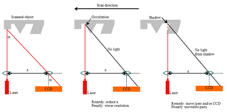
Figure 4. (left panel) Laser scanning to obtain 3D information about the target object; (middle panel) occultation occurs when there is no direct line of sight between the illuminated point and the camera; (right panel) shadowing occurs when there is no direct line of sight between the laser and the point intended for illumination.

The scanned object in Figure 4 moves to the left with respect to the stationary laser and CCD camera. The laser beam is perpendicular to the baseline x. The left panel shows a situation where the laser-camera system can make a successful distance measurement, whereas the middle and right panels show cases where they cannot. Occultation, depicted in the middle panel, occurs when the light from the reflection point cannot reach the camera because parts of the object block the way. Shadowing, depicted in the right panel, occurs when light from the laser cannot reach the point to be scanned. A remedy to reduce occultation is a decrease of x with the penalty of increased δd. To reduce or eliminate shadowing, the orthogonality of the beam and the baseline may have to be relaxed. This would involve moveable parts in the illumination/detection system — a major disadvantage.

Another disadvantage of point-by-point scanning is a slow rate of image acquisition, and a tradeoff between this rate and the density of points. The latter affects the spatial resolution of the scanned scene. The next section discusses a faster approach.

Structured light

Figure 5. The concept of structured light approach of obtaining 3D information.

Point-by-point scanning is time consuming. A faster approach, albeit involving more complex data analysis and computing, is to illuminate the target object with structured light — a single line or a pattern of lines (e.g., parallel lines or a grid) — and use a 2D image sensor to detect the reflected pattern. Figure 5 illustrates the concept. In the left panel, the light projector casts a straight luminous line on the flat target. Here, the CCD image of the projection is also a straight line. In the right panel, the projected luminous line is comparable in size to the structural features of the target object (a cube, in this example). The image of the projection will not be a straight line (for most of the projector/camera configurations); for the fixed projector/camera locations, the shape of the image depends on the shape of the object. A mathematical algorithm can be developed to deduce the shape of the target given the geometry of the input and imaged structured light.

In practical applications of structured light, there are two approaches of generating structured light. The first uses two wide-beam lasers whose light generates an interference pattern, free of geometrical distortions, on the target. By changing the angle between the two beams, a wide range of patterns with large optical depth can be generated. The implementation of this approach is difficult because the geometry of the interference pattern is very sensitive to the relative orientation of the two beams. Another disadvantage is high cost. The second arrangement of illumination, less expensive than the first, uses a video projector, which projects a luminous pattern from, for example, a liquid crystal display, onto the target using lenses and mirrors. The tradeoff for the lower cost is a greater degree of geometrical distortions in the projected structured light and pixelated edges of the pattern if the image comes from a pixelated device such as a liquid crystal display. When analyzing the data, the geometrical distortions introduced by the projector and the detection system must be corrected for, which makes the mathematical algorithm more complex. Practical applications of structured light are diverse, ranging from video gaming (Microsoft Kinect), through fashion industry (made-to-measure apparel production), to forensics (fingerprint acquisition).

Depth from defocus

A technique known as "depth from defocus" is a variant of structured light. It relies on a mathematical relationship between the perpendicular distance from a target to a lens (so) and the distance from the lens to the image of the target formed by the lens (si). For a thin lens with a focal length ƒ, this relationship is given by the well-known thin lens equation:

Equation 5

\frac{1}{s_{o}} + \frac{1}{s_{i}} = \frac{1}{f}

Figure 6. Concept of depth from defocus. Adapted from Nayar et al. (1995).

Figure 6 illustrates the concept. Consider point P on the target (tip of the arrow), which is an unknown perpendicular distance so from the lens. The lens creates a real image of the point at P′, which a CCD camera located in the plane If would record as being in focus. Measuring the distance between If and the lens, si, and substituting the value into Equation 5 yields the unknown distance so. An extended object can be thought of as a superposition of an infinite number of points; therefore, repeating the above procedure to enough target points produces a depth map of the target. The points can be selected from the target itself or be projected onto the target (structured light) as described in a previous section.

Although conceptually correct, the method described in the previous paragraph (which is equivalent to point-by-point scanning) is impractical when applied to a target with a rugged and complex surface because the camera (or the lens) must be moved to bring a sampled point into focus. This is time consuming. In addition, the system has moveable parts and, thus, an elevated probability of mechanical failure.

An alternative approach uses two CCD cameras placed in planes I1 and I2 to obtain two images of the target. The appearance of point P is out of focus in both CCD images, and the degree of defocus depends on the values of α and β. An aperture stop placed in the focal plane on the side of the object ensures that the location of P′ (center of the blur disk) has the same coordinate in both CCD images regardless of the values of α and β. A mathematical algorithm determines so from the two images for point P and, using the same CCD images, for any number of preselected points on the target. A 3D map of the target results from two defocused CCD images without involving moveable parts. For further details, an interested reader is referred to Nayar et al. (1995) who give an in-depth discussion of the method, describe the key elements of the mathematical analysis required to extract depth information from two out-of-focus images, and present a functioning system capable of producing depth maps at the video rate of 30 Hz.

Time of flight (TOF)

Direct time of flight

In the direct TOF techniques, the time of flight is measured directly with a clock. Figure 7 depicts a possible setup.

Figure 7. Possible setup for time-of-flight distance measurement using a pulsed laser. This setup is suitable for distances on the order of kilometers. Adapted from Petrie & Toth (2009).

The laser emits pulses of light of wavelength λ₀, duration t_p, and repetition period T. A beam splitter directs some fraction of the light to a "fast" photodetector such as a PIN photodiode or avalanche photodiode; the output pulse of the photodetector provides the "start" pulse to a timer (clock). The remaining fraction of light passes through the collimation and beam expander optics and travels to the target in a medium with index of refraction n. After reflection from the target, some fraction of the light is collected by the telescope and directed towards the second "fast" photodetector. The photodetector produces the "stop" pulse to the timer. Though not shown in the figure, the actual setup would also have bandpass filters centered on λ₀ to reduce background light. If the time between start and stop pulses is t, then the distance d to the target is given by:

Equation 6

d = c t / 2 n

The uncertainty δ_d in the measured distance is primarily due to the uncertainty δ_t of the measured time t and is given by Equation 7:

Equation 7

δ_{d} \approx \frac{c δ_{t}}{2 n}

There are several sources of δ_t. Figure 8 shows the relationship between the start and stop pulses that trigger the timer.

Figure 8. Relationship between the start and stop pulses. Adapted from Petrie & Toth (2009).

The amplitude A_T of the start pulse — voltage or current produced by the photodetector — is controlled by the amount of light siphoned to the detector by the beam splitter. The amplitude A_R of the stop pulse depends on the amount of reflected light collected by the telescope. For a given telescope aperture size, this quantity of light depends on the light power in the laser pulse, the distance to the target, and the characteristics of the reflection (i.e., the target's color, orientation, surface smoothness, etc.). Although A_T can be adjusted by the beam splitter so that A_T = AR, in most situations A_T ≠ A_R with the former being larger.

The timer starts and then stops if the leading edges of the start and stop pulses reach certain predetermined levels of voltage or current. In practice, these levels could be set to some fixed fraction of the peak values. Because of time jitter in the photodetectors, variations in rise times, and electrical noise in the pulses, the timer does not measure a constant TOF t — thus there is δ_t — even though the target is stationary. Although the laser also introduces time jitter into the repetition period, this jitter does not contribute to δ_t. Using 1 ns as a reasonable time jitter for each photodetector, δ_d ≈ 21 cm. For a target 1 m away, the jitter causes an almost 25% fractional error; reducing this error requires photodetectors with smaller jitter. All else being the same, the fractional error decreases with increasing distance to the target. In practice, however, all else is usually not the same. For a given telescope aperture size and laser light power, as the distance increases, the amount of reflected light illuminating the photodetector decreases, causing the stop pulse to be more noisy and thus contributing to δ_t.

As shown in Figure 8, the repetition period T of the laser pulses should not be smaller than T_min = t + t_p or the maximum repetition frequency not be greater than ƒ_max = 1/T_min. For a target 100 m away, t = 0.67 μs. If t_p << t, ƒ_max = 1.5 MHz. The repetition frequency decreases linearly with increasing d. This has no consequences if the target is stationary, but if it is not, the resolution of its position as a function of time decreases with d. The resolution is degraded even further if a setup uses a light chopper instead of a high-power pulsed laser; here, t_p can be comparable to t.

Indirect time of flight

Phase comparison method

Figure 9 illustrates the concept of measuring distance to a target using the phase shift φ between the intensity-modulated transmitted and received waves. The transmitter emits light whose intensity is modulated (sinusoidal modulation is common) by either the transmitter itself (if it is a laser or LED) or an optical system such as Kerr cell, Pockels cell, or a mechanical shutter. The light does not need to be monochromatic and polarized. The light reflects from the target and arrives at the receiver having a phase shift with respect to the transmitted wave of φ, which can have a value between 0 and 2π.

Figure 9. Phase comparison method of measuring distance. The emitted light is intensity-modulated (assumed sinusoidal) with the modulation wavelength λ_m. Adapted from Petrie & Toth (2009).

If the wavelength of the sinusoidal modulation is λ_m, Equation 8 gives the corresponding phase shift, while Equation 9 gives the distance to the target.

Equation 8

Δ λ_{m} = \frac{Φ λ_{m}}{2 π} = \frac{c Φ}{2 π f_{m}}

Equation 9

d = \frac{1}{2} (M λ_{m} + ∆ λ_{m})

In the above equations, ƒ_m is the frequency of modulation and M is an integer that is equal to the number of full modulation wavelengths in the distance 2d as illustrated in Figure 10.

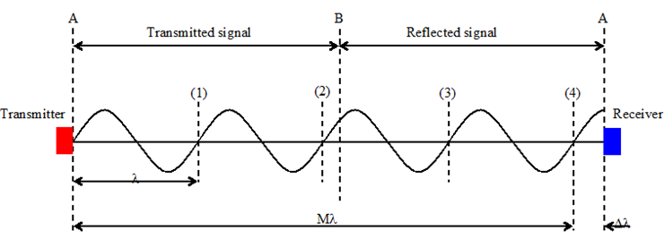
Figure 10. In this example, there are four full modulation wavelengths (M = 4) in the roundtrip distance from the transmitter to the target and back to the transmitter. Adapted from Petrie & Toth (2009).

For the sake of clarity, the roundtrip distance from the transmitter (at location A) to the target (at location B) and back to the receiver (at location A) has been "unfolded." In the example illustrated by the figure, M = 4. If M is not known, the absolute distance to the target cannot be determined, i.e., the distance is ambiguous. If M=0, the maximum unambiguous distance that can be measured is d_max = ^λ_m/₂ = ^c/_{2ƒ_m}. For ƒ_m = 10 MHz, d_max = 15 m. Decreasing modulation frequency increases the maximum unambiguous distance; however, doing so also increases the uncertainty δ_d in the measured distance. The uncertainty is given by:

Equation 10

δ_{d} = \frac{c δ_{Φ}}{4 π f_{m}}

where δ_Φ is the uncertainty in the measured phase difference between the emitted and received waves. For δ_Φ ≈ 1° and ƒ_m = 10 MHz, δ_d ≈ 4 cm, implying a fractional error of 0.3%.

TOF 3D imaging

A point-by-point scanning of a scene using either a direct or indirect TOF technique discussed above provides depth of the scene. Prior to the mid-1990s, a 3D camera employing either of these two techniques required a mechanical scanning system to sample an array of points on the target surface. One limitation of such an arrangement is a compromise between the frame rate and density of sampled points, where the former affects the temporal accuracy of depth measurement for a moving target, whereas the latter affects the spatial resolution of the features on the target. This compromise could have been lessened if it were possible to measure simultaneously all of the distances to an array of points on the target surface. This is now possible.

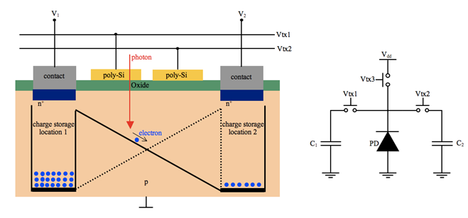
Figure 11. A simplified structure of a PMD (left panel) and its equivalent electrical circuit (right panel).

The breakthrough is the development of a CMOS-architecture imaging array where each pixel is a Photonic Mixer Device (PMD). The left panel in Figure 11 depicts a simplified structure of a PMD. An internal electric field directs the photogenerated charge carrier (electron) to one of the two charge storage locations. Two external signals Vtx1 and Vtx2 control the strength and direction of the electric field and, therefore, they also control how much charge each storage location receives in response to incident light. The output signals V₁ and V₂ are a measure of how much charge has been accumulated in locations 1 and 2, respectively. The right panel of Figure 11 shows a simplified electrical equivalent circuit of a PMD. The main components are a photodiode (generator of photo-charge), two capacitors (charge storage locations), and switches (responsible for directing the photo-charge to the appropriate capacitors).

In one common arrangement, a 3D camera system illuminates the scene with an intensity-modulated infrared light. The optics of the system creates an image of the scene on the array of PMD pixels. For each pixel, the system determines an autocorrelation function between the electrical signal that modulates the emitted light and the electrical signals coming from the two capacitors. Sampling the resulting function four times per period gives the phase shift, strength of the returned signal, and the background level using well-known mathematical relations. The distance is proportional to the phase shift.

In the second arrangement, a 3D camera system illuminates the scene with a pulse of infrared light of duration T₀ (30 — 50 ns) while simultaneously making the pixels sensitive to light for the duration of 2T₀. During the first half of 2T₀, only one of the two capacitors collects the charge, whereas during the second half, only the second capacitor does. The distance imaged by a pixel derives from the relative amounts of charge collected by each of the two capacitors and is given by:

Equation 11

d = \frac{1}{2} c T_{0} \frac{V_{2}}{V_{1} + V_{2}}

where V₁ and V₂ are the voltages developed on the two capacitors, respectively, in response to accumulated charge. For a given pulse duration, the maximum distance that can be measured is d_max = 1/2cT₀, corresponding to V₁ = 0 (no charge collected on the first capacitor). The uncertainty δ_d in the measured distance by a pixel increases linearly with T₀ and decreases as inverse square root with increasing signal-to-noise (S/N) ratio, $δ_{d} \propto \frac{\frac{1}{2} c T_{0}}{\sqrt{\frac{S}{N}}}$ . The noise N in the equation is a square root of the sum in quadrature of the signal (photon) shot noise, dark current shot noise, background shot noise, and read noise. The above equation assumes that the target is at 1/2 d_max so that the amount of charge accumulated by each capacitor is the same. If the photon shot noise is dominant, δ_d reduces to cT₀/4√N_e, where N_e is the number of photoelectrons accumulated together by the two capacitors.

Interferometry

The TOF techniques discussed above work well for distant targets (meters away or more) but become progressively less accurate as the distance becomes smaller (meter and less). They eventually become inapplicable for distances on the order of mm or less, for example, comparable to the wavelength of light. In the case of a direct TOF technique, there is no clock capable of measuring roundtrip time of about 7 fs for 1 μm distance. To measure this distance with a phase-comparison, indirect TOF technique using intensity-modulated light, the required modulation frequency would have to be about 2×1014 Hz, while the duration of a pulse in the 3D PMD camera would have to be about 7 fs. None of the above technical requirements are easily attainable, but why not use the wavelength of light itself to probe distances on the micron scale? The Michelson-Morley interferometer allows just that.

Michelson-Morley interferometer

Figure 12 depicts the basic design of the Michelson-Morley interferometer. The beam splitter divides the incoming continuous-wave light from a laser (coherent and polarized light) so that one portion travels to the stationary mirror — serving as the reference — and the other portion travels to the target.

Figure 12. Michelson-Morley interferometer.

After the reflections, the two beams are directed to the photodetector where they are made to interfere. The output of the photodetector is proportional to the optical intensity of the combined light and given by:

Equation 12

I = I_{1} + I_{2} + 2 \sqrt{I_{1} I_{2}} \cos \{\frac{2 π (2 d- 2 x)}{λ}\}

Here, I₁ is the intensity of, for example, the reference beam (from the stationary mirror), and I₂ is the intensity of the beam from the target. Equation 12 assumes that the light is spatially and temporally coherent and that the interfering beams have not acquired a net phase shift due to reflections. Assuming for the sake of simplicity that I₁ = I₂, Equation 12 shows that the combined intensity I varies from 0 to 4I₁ depending on the value of $d - x$ . If $d - x = \frac{n λ}{2} (n = 0,1,2.. .)$ , a constructive interference occurs and the combined intensity is 4I₁. For $d - x = \frac{n λ}{2} + \frac{λ}{4}$ , a destructive interference occurs and I = 0. Suppose that the location x of the reference mirror is such that the photodetector registers a maximum when the target is at location d. If the target now moves either away or towards the beam splitter, the photodetector will register a minimum and a maximum each time the target moves through a point that is $\frac{n λ}{2} + \frac{n λ}{4}$ and $\frac{n λ}{2}$ , respectively, away from the starting point, where n increases by 1, starting from 0, at each crossing. Counting the crossings makes it possible to determine the distance the target has moved to an accuracy of about λ/4.

If the interfering beams in the Michelson-Morley interferometer have acquired a relative phase shift of π, or λ/2, due to reflections, the conditions for the constructive and destructive interference that were stated in the previous paragraph interchange. In the case where d≠x, the completely constructive (I = 4I₁) and completely destructive interference (I = 0) requires light to be temporally coherent because the interfering light at a given instant has been emitted — by the laser — at different times. Temporal coherence measures the correlation between the light wave at a given instant and at a later (or earlier) time. If the light is perfectly monochromatic, the correlation at t and t + T, where T is the wave's period, is 1. If the correlation is not 1, the wave cannot be monochromatic. Therefore, temporal coherence is a measure of how monochromatic a light wave is. Equation 13 defines visibility ν, where I_max and I_min are the maximum and minimum intensities for the interfering light:

Equation 13

v = \frac{I_{m a x} - I_{m i n}}{I_{m a x} + I_{m i n}}

For a perfect temporal coherence, ν = 1 and for a perfect incoherence, ν = 0.

Optical coherence tomography

Optical coherence tomography (OCT) is a technique to generate "slice" images in lateral and longitudinal directions of a three-dimensional target using light with a finite temporal coherence, such as from a superluminous light emitting diode (SLED). Figure 13 shows the basic setup for this technique. OCT is widely used in life sciences because it is capable of a noninvasive, in vivo, and in situ microimaging of biological tissue.

Figure 13. The basic setup for time-domain optical coherence tomography.

The basic setup for time-domain OCT resembles the Michelson-Morley interferometer. The light from a limited-coherence source divides into two paths or arms. The first arm leads to a moveable mirror and the second to a target sample. After reflecting from the mirror and structural features in the sample, the returning light combines and interferes on the surface of a photodetector. To perform a longitudinal scan of the sample, the output of the photodetector is recorded while the mirror smoothly moves at a known and controlled rate in one direction. Therefore, the instantaneous value of the photodetector output correlates with the instantaneous position of the mirror and may look like the left panel of Figure 14.

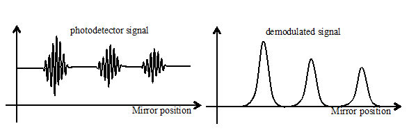
Figure 14. (left panel) A possible photodetector output as a function of the moveable mirror position for three reflection sites, as depicted in Figure 13. (right panel) The signal in the left panel after demodulation.

Here, the photodetector signal shows three distinct interference patterns that would result if there were three distinct reflection sites, as shown in Figure 13 (three strands in the sample). The coherence length of the light source determines the spatial width of a single interference pattern. The right panel shows the signal after demodulation. The relative locations of the three strands correspond to the locations of the peaks of the three distinct peaks. The width of a given strand (reflection site) affects the width of its corresponding demodulated signal.

The longitudinal (or axial) resolution of OCT is $δ_{r} = 0.44 \frac{λ_{0}^{2}}{△ λ}$ , whereas the lateral (or transverse) resolution is $δ_{z} = \frac{4 λ_{0} f}{π D}$ . In the equations, λ₀ is the central wavelength, Δλ is the bandwidth of the light source, ƒ is the focal length of lens L₂ (see Figure 13), and D is the diameter of the beam of light at lens L₂. Most OCT systems use a light source with λ₀ = 1300 nm and Δλ = 100 nm which imply δ_r ≈ 7μm. A typical transverse resolution is in the 10 — 25 μm range.

The time-domain OCT setup has some drawbacks: it contains moveable parts, which make the system slow and, thus, poorly performing in in vivo scans. Frequency- or Fourier-domain OCT is an alternative approach whose setup does not use moving parts, is faster, and yields a higher signal-to-noise ratio. There are two practical realizations of frequency-domain OCT. The first uses a wide-band illumination (similar to the one in time-domain OCT), fixed diffraction grating, and a CCD camera. The back-reflected light is the input to the grating, whereas the CCD camera records the resulting interference pattern, which is a function of the target's structure. The second possible setup uses a narrow-band, frequency-swept, and continuous-wave light source (e.g., tunable laser) and a single-element photodetector for detecting time-dependent interference signals. Although more costly to implement, frequency-domain OCT outperforms its time-domain counterpart; for a side-by-side comparison, refer to Leitgeb, Hitzenberger, and Fercher (2003).

References

R. Leitgeb, C. K. Hitzenberger, and A. F. Fercher, "Performance of Fourier-domain vs. time domain optical coherence tomography," Opt. Express 11, 889 (2003).
S. K. Nayar, M. Noguchi, M. Watanabe and Y. Nakagawa, "Focus Range Sensors" in Robotics Research, the Seventh International Symposium, edited by Georges Giralt and Gerhard Hirzinger, p. 378-390. Springer 978-1-4471-1254-9.
G. Petrie and C. K. Toth 2009, Topographic Laser Ranging and Scanning, edited by Jie Shan and Charles K. Toth, CRC Press, p. 1-27.